
This document describes various aspects of accessing data in an Adabas database with Natural.
The following topics are covered:
See also Database Management in Profile Parameters Grouped by Category (Parameter Reference documentation) for an overview of the Natural profile parameters that apply when Natural is used with Adabas.
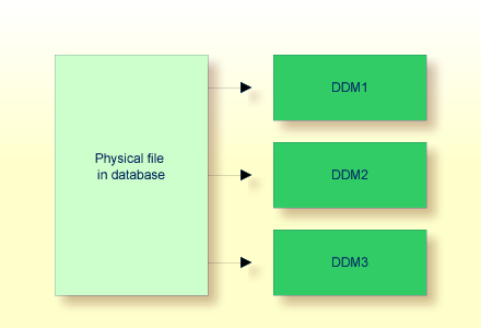
For Natural to be able to access a database file, a logical definition of the physical database file is required. Such a logical file definition is called a data definition module (DDM).
This section covers the following topics:
The data definition module contains information about the individual fields of the file - information which is relevant for the use of these fields in a Natural program. A DDM constitutes a logical view of a physical database file.
For each physical file of a database, one or more DDMs can be
defined. And for each DDM one or more data views can be defined as described
View
Definition in the DEFINE DATA statement
documentation and explained in the section Defining a Database
View.
DDMs are defined by the Natural administrator with Predict (or, if Predict is not available, with the corresponding Natural function).
Use the system command
SYSDDM to invoke the SYSDDM utility.
The SYSDDM utility is used to perform all functions needed for the
creation and maintenance of Natural data definition modules.
For further information on the SYSDDM
utility, see the section SYSDDM Utility in the
Editors documentation.
For each database field, a DDM contains the database-internal
field name as well as the "external" field name, that is, the name
of the field as used in a Natural program. Moreover, the formats and lengths of
the fields are defined in the DDM, as well as various specifications that are
used when the fields are output with a DISPLAY or
WRITE statement (column headings, edit masks, etc.).
For the field attributes defined in a DDM, refer to Using the DDM Editor in the section SYSDDM Utility of the Editors documentation.
If you do not know the name of the DDM you want, you can use the
system command LIST DDM to get a list of
all existing DDMs that are available in the current library. From the list, you
can then select a DDM for display.
To display a DDM whose name you know, you use the system command
LIST DDM ddm-name.
For example:
LIST DDM EMPLOYEES
A list of all fields defined in the DDM will then be displayed, along with information about each field. For the field attributes defined in a DDM, refer to SYSDDM Utility in the Editors documentation.
Adabas supports array structures within the database in the form of multiple-value fields and periodic groups.
This section covers the following topics:
A multiple-value field is a field which can have more than one value (up to 65534, depending on the Adabas version and definition of the FDT) within a given record.
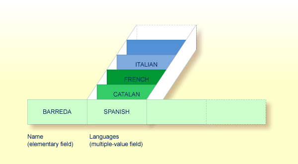
Assuming that the above is a record in an employees file, the first field (Name) is an elementary field, which can contain only one value, namely the name of the person; whereas the second field (Languages), which contains the languages spoken by the person, is a multiple-value field, as a person can speak more than one language.
A periodic group is a group of fields (which may be elementary fields and/or multiple-value fields) that may have more than one occurrence (up to 65534, depending on the Adabas version and definition of the field definition table (FDT)) within a given record.
The different values of a multiple-value field are usually called "occurrences"; that is, the number of occurrences is the number of values which the field contains, and a specific occurrence means a specific value. Similarly, in the case of periodic groups, occurrences refer to a group of values.
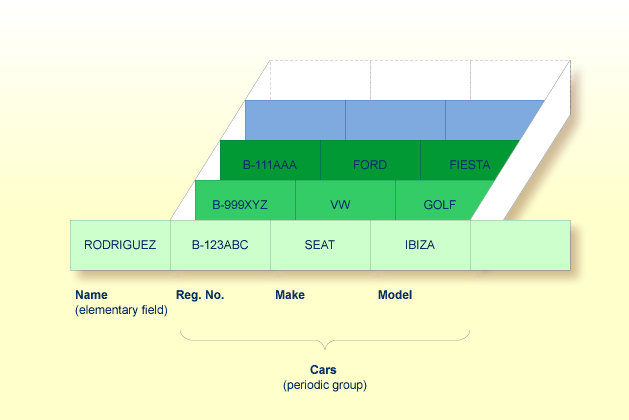
Assuming that the above is a record in a vehicles file, the first field (Name) is an elementary field which contains the name of a person; Cars is a periodic group which contains the automobiles owned by that person. The periodic group consists of three fields which contain the registration number, make and model of each automobile. Each occurrence of Cars contains the values for one automobile.
To reference one or more occurrences of a multiple-value field or a periodic group, you specify an "index notation" after the field name.
The following examples use the multiple-value field
LANGUAGES and the periodic group CARS from the
previous examples.
The various values of the multiple-value field
LANGUAGES can be referenced as follows.
| Example | Explanation |
|---|---|
LANGUAGES (1)
|
References the first value
(SPANISH).
|
LANGUAGES (X)
|
The value of the variable X determines the value to be referenced. |
LANGUAGES (1:3)
|
References the first three values
(SPANISH, CATALAN and FRENCH).
|
LANGUAGES (6:10) |
References the sixth to tenth values. |
LANGUAGES (X:Y)
|
The values of the variables X and
Y determine the values to be referenced.
|
The various occurrences of the periodic group CARS
can be referenced in the same manner:
| Example | Explanation |
|---|---|
CARS (1) |
References the first occurrence
(B-123ABC/SEAT/IBIZA).
|
CARS (X)
|
The value of the variable X determines
the occurrence to be referenced.
|
CARS (1:2)
|
References the first two occurrences
(B-123ABC/SEAT/IBIZA and B-999XYZ/VW/GOLF).
|
CARS (4:7)
|
References the fourth to seventh occurrences. |
CARS (X:Y)
|
The values of the variables X and
Y determine the occurrences to be referenced.
|
An Adabas array can have up to two dimensions: a multiple-value field within a periodic group.
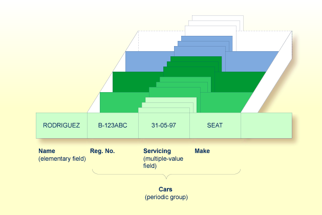
Assuming that the above is a record in a vehicles file, the first field (Name) is an elementary field which contains the name of a person; Cars is a periodic group, which contains the automobiles owned by that person. This periodic group consists of three fields which contain the registration number, servicing dates and make of each automobile. Within the periodic group Cars, the field Servicing is a multiple-value field, containing the different servicing dates for each automobile.
To reference one or more occurrences of a multiple-value field within a periodic group, you specify a "two-dimensional" index notation after the field name.
The following examples use the multiple-value field
SERVICING within the periodic group CARS from the
example above. The various values of the multiple-value field can be referenced
as follows:
| Example | Explanation |
|---|---|
SERVICING (1,1)
|
References the first value of SERVICING
in the first occurrence of CARS (31-05-97).
|
SERVICING (1:5,1)
|
References the first value of SERVICING
in the first five occurrences of CARS.
|
SERVICING (1:5,1:10) |
References the first ten values of
SERVICING in the first five occurrences of
CARS.
|
It is sometimes necessary to reference a multiple-value field or a
periodic group without knowing how many values/occurrences exist in a given
record. Adabas maintains an internal count of the number of values in each
multiple-value field and the number of occurrences of each periodic group. This
count may be read in a READ statement by specifying
C* immediately before the field name.
The count is returned in format/length N3. See Referencing the Internal Count for a Database Array for further details.
| Example | Explanation |
|---|---|
C*LANGUAGES |
Returns the number of values of the multiple-value
field LANGUAGES.
|
C*CARS |
Returns the number of occurrences of the periodic
group CARS.
|
C*SERVICING (1) |
Returns the number of values of the multiple-value
field SERVICING in the first occurrence of a periodic group
(assuming that SERVICING is a multiple-value field within a
periodic group.)
|
To be able to use database fields in a Natural program, you must specify the fields in a database view.
In the view, you specify the name of the data definition module (see Data Definition Modules - DDMs) from which the fields are to be taken, and the names of the database fields (see Field Definitions) themselves (that is, their long names, not their database-internal short names).
The view may comprise an entire DDM or only a subset of it. The order of the fields in the view need not be the same as in the underlying DDM.
As described in the section Statements for Database
Access, the view name is used in the statements
READ, FIND, HISTOGRAM to determine which
database is to be accessed.
For further information on the complete syntax of the view
definition option or on the definition/redefinition of a group of fields, see
View
Definition in the description of the DEFINE
DATA statement in the Statements documentation.
Basically, you have the following options to define a database view:
Inside the Program
You can define a database view inside the program, that is,
directly within the DEFINE
DATA statement of the program.
Outside the Program
You can define a database view outside the program, that is, in
a separate object: either a
local data
area (LDA) or a
global data
area (GDA), with the DEFINE DATA statement of the
program referencing that data area.
 To define a database view inside the program
At Level 1, specify the view name as follows:
1 view-name VIEW OF ddm-name
where view-name is the
name you choose for the view, ddm-name
is the name of the DDM from which the fields specified in the view are
taken.
At Level 2, specify the names of the database fields from the DDM.
In the illustration below, the name of the view is
ABC, and it comprises the fields NAME,
FIRST-NAME and PERSONNEL-ID from the DDM
XYZ.
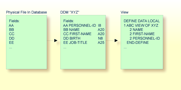
In the view, the format and length of a database field need not be specified, as these are already defined in the underlying DDM.
Sample Program:
In this example, the
view-name is VIEWEMP, and
the ddm-name is EMPLOYEES,
and the names of the database fields taken from the DDM are NAME,
FIRST-NAME and PERSONNEL-ID.
DEFINE DATA LOCAL 1 VIEWEMP VIEW OF EMPLOYEES 2 NAME 2 FIRST-NAME 2 PERSONNEL-ID 1 #VARI-A (A20) 1 #VARI-B (N3.2) 1 #VARI-C (I4) END-DEFINE ...
To define a database view outside the program
In the program, specify:
DEFINE DATA LOCAL
USING <data-area-name>
END-DEFINE
...
where data-area-name
is the name you choose for the local or global data area, for example,
LDA39.
In the data area to be referenced:
At Level 1 in the Name column, specify the
name you choose for the view, and in the Miscellaneous column, the
name of the DDM from which the fields specified in the view are taken.
At Level 2, specify the names of the database fields from the DDM.
Example LDA39:
In this example, the view name is VIEWEMP,
the DDM name is EMPLOYEES, and the names of the database fields
taken from the DDM are PERSONNEL-ID, FIRST-NAME and
NAME.
I T L  Name                             F Length     Miscellaneous
All -- -------------------------------- - ---------- ------------------------->
  V  1 VIEWEMP                                       EMPLOYEES
     2 PERSONNEL-ID                     A          8
     2 FIRST-NAME                       A         20
     2 NAME                             A         20
     1 #VARI-A                          A         20
     1 #VARI-B                          N        3.2
     1 #VARI-C                          I          4
To read data from a database, the following statements are available:
| Statement | Meaning |
|---|---|
READ
|
Select a range of records from a database in a specified sequence. |
FIND
|
Select from a database those records which meet a specified search criterion. |
HISTOGRAM
|
Read only the values of one database field, or determine the number of records which meet a specified search criterion. |
The following topics are covered:
The READ
statement is used to read records from a database. The records can be retrieved
from the database
in the order in which they are physically stored in the
database (READ IN PHYSICAL
SEQUENCE), or
in the order of Adabas Internal Sequence Numbers (READ BY ISN), or
in the order of the values of a descriptor field (READ IN LOGICAL
SEQUENCE).
In this document, only READ IN LOGICAL SEQUENCE is
discussed, as it is the most frequently used form of the READ
statement.
For information on the other two options, please refer to the
description of the READ
statement in the Statements documentation.
The basic syntax of the READ statement is:
READ
view IN LOGICAL SEQUENCE
BY descriptor
|
or shorter:
READ
view LOGICAL BY
descriptor
|
- where
view
|
is the name of a view defined in the
DEFINE DATA
statement and as explained in Defining a Database
View.
|
descriptor
|
is the name of a database field defined in that view. The values of this field determine the order in which the records are read from the database. |
If you specify a descriptor, you need not specify the
keyword LOGICAL:
READ
view BY
descriptor
|
If you do not specify a descriptor, the records will be read in
the order of values of the field defined as default descriptor (under
Default Sequence) in the DDM. However, if you specify no descriptor,
you must specify the keyword
LOGICAL:
READ
view LOGICAL
|
** Example 'READX01': READ
************************************************************************
DEFINE DATA LOCAL
1 MYVIEW VIEW OF EMPLOYEES
  2 NAME
  2 PERSONNEL-ID
  2 JOB-TITLE
END-DEFINE
*
READ (6) MYVIEW BY NAME
  DISPLAY NAME PERSONNEL-ID JOB-TITLE
END-READ
END
Output of Program READX01:
With the READ statement in this example,
records from the EMPLOYEES file are read in alphabetical order of
their last names.
The program will produce the following output, displaying the information of each employee in alphabetical order of the employees' last names.
Page      1                                                  04-11-11  14:15:54

        NAME         PERSONNEL          CURRENT
                        ID             POSITION
-------------------- --------- -------------------------

ABELLAN              60008339  MAQUINISTA
ACHIESON             30000231  DATA BASE ADMINISTRATOR
ADAM                 50005800  CHEF DE SERVICE
ADKINSON             20008800  PROGRAMMER
ADKINSON             20009800  DBA
ADKINSON             2001100
If you wanted to read the records to create a report with the
employees listed in sequential order by date of birth, the appropriate
READ statement would be:
READ MYVIEW BY BIRTH
You can only specify a field which is defined as a "descriptor" in the underlying DDM (it can also be a subdescriptor, superdescriptor, hyperdescriptor or phonetic descriptor or a non-descriptor).
As shown in the previous example program, you can limit the
number of records to be read by specifying a number in parentheses after the
keyword READ:
READ (6) MYVIEW BY NAME
In that example, the READ statement would read no
more than 6 records.
Without the limit notation, the above READ
statement would read all records from the EMPLOYEES file
in the order of last names from A to Z.
The READ
statement also allows you to qualify the selection of records based on the
value of a descriptor field. With an
EQUAL TO/STARTING
                        				  FROM
option in the BY clause, you can specify
the value at which reading should begin. (Instead of using the keyword
BY, you may specify the keyword WITH, which would
have the same effect). By adding a
THRU/ENDING
                        				  AT
option, you can also specify the value in the logical
sequence at which reading should end.
For example, if you wanted a list of those employees in the
order of job titles starting with TRAINEE and continuing on to
Z, you would use one of the following statements:
READ MYVIEW WITH JOB-TITLE = 'TRAINEE'
READ MYVIEW WITH JOB-TITLE STARTING FROM 'TRAINEE'
READ MYVIEW BY JOB-TITLE = 'TRAINEE'
READ MYVIEW BY JOB-TITLE STARTING FROM 'TRAINEE'
Note that the value to the right of the equal sign (=) or
STARTING
                        				  FROM
option must be enclosed in apostrophes. If the value is
numeric, this text notation is
not required.
The sequence of records to be read can be even more closely
specified by adding an end limit with a
THRU/ENDING
                        				  AT
clause.
To read just the records with the job title
TRAINEE, you would specify:
READ MYVIEW BY JOB-TITLE STARTING FROM 'TRAINEE' THRU 'TRAINEE'
READ MYVIEW WITH JOB-TITLE EQUAL TO 'TRAINEE'
                           ENDING AT 'TRAINEE'
To read just the records with job titles that begin with
A or B, you would specify:
READ MYVIEW BY JOB-TITLE = 'A' THRU 'C'
READ MYVIEW WITH JOB-TITLE STARTING FROM 'A' ENDING AT 'C'
The values are read up to and including the value specified
after THRU/ENDING
AT. In the two examples above, all records with job titles
that begin with A or B are read; if there were a job
title C, this would also be read, but not the next higher value
CA.
The WHERE clause may be
used to further qualify which records are to be read.
For instance, if you wanted only those employees with job titles
starting from TRAINEE who are paid in US currency, you would
specify:
READ MYVIEW WITH JOB-TITLE = 'TRAINEE'
            WHERE CURR-CODE = 'USD'
The WHERE clause can also be used with the
BY clause as
follows:
READ MYVIEW BY NAME
            WHERE SALARY = 20000
The WHERE clause differs from the
BY clause in two
respects:
The field specified in the WHERE clause need
not be a descriptor.
The expression following the WHERE option is a
logical condition.
The following logical operators are possible in a
WHERE clause:
EQUAL |
EQ |
= |
NOT EQUAL TO |
NE |
¬= |
LESS THAN |
LT |
< |
LESS THAN OR EQUAL
TO |
LE |
<= |
GREATER THAN |
GT |
> |
GREATER THAN OR EQUAL
TO |
GE |
>= |
The following program illustrates the use of the
STARTING FROM,
ENDING AT and WHERE clauses:
** Example 'READX02': READ  (with STARTING, ENDING and WHERE clause)
************************************************************************
DEFINE DATA LOCAL
1 MYVIEW VIEW OF EMPLOYEES
  2 NAME
  2 JOB-TITLE
  2 INCOME     (1:2)
    3 CURR-CODE
    3 SALARY
    3 BONUS    (1:1)
END-DEFINE
*
READ (3) MYVIEW WITH  JOB-TITLE
STARTING FROM 'TRAINEE' ENDING AT 'TRAINEE'
                WHERE CURR-CODE (*) = 'USD'
  DISPLAY NOTITLE NAME / JOB-TITLE 5X INCOME (1:2)
  SKIP 1
END-READ
END
Output of Program READX02:
         NAME                            INCOME
         CURRENT
        POSITION              CURRENCY   ANNUAL     BONUS
                                CODE     SALARY
-------------------------     -------- ---------- ----------

SENKO                         USD           23000          0
TRAINEE                       USD           21800          0

BANGART                       USD           25000          0
TRAINEE                       USD           23000          0

LINCOLN                       USD           24000          0
TRAINEE                       USD           22000          0
See the following example program:
The following topics are covered:
The FIND
statement is used to select from a database those records which meet a
specified search criterion.
The basic syntax of the FIND statement is:
FIND RECORDS IN
view WITH
field = value
|
or shorter:
FIND
view WITH
field = value
|
- where
view
|
is the name of a view as defined in the
DEFINE DATA
statement and as explained in Defining a Database
View.
|
field
|
is the name of a database field as defined in that view. |
You can only specify a
field which is defined as a
"descriptor" in the underlying DDM (it can also be a subdescriptor,
superdescriptor, hyperdescriptor or phonetic descriptor).
For the complete syntax, refer to the
FIND statement
documentation.
In the same way as with the READ statement
described above, you can
limit the number of records to be processed by specifying a number in
parentheses after the keyword FIND:
FIND (6) RECORDS IN MYVIEW WITH NAME = 'CLEGG'
In the above example, only the first 6 records that meet the search criterion would be processed.
Without the limit notation, all records that meet the search criterion would be processed.
Note:
If the FIND statement contains a
WHERE
clause (see below), records which are rejected as a result of the
WHERE clause are not counted against the limit.
With the WHERE clause of the
FIND statement, you can
specify an additional selection criterion which is evaluated after a
record (selected with the WITH clause) has been
read and before any processing is performed on the record.
** Example 'FINDX01': FIND (with WHERE)
************************************************************************
DEFINE DATA LOCAL
1 MYVIEW VIEW OF EMPLOYEES
  2 PERSONNEL-ID
  2 NAME
  2 JOB-TITLE
  2 CITY
END-DEFINE
*
FIND MYVIEW WITH CITY = 'PARIS'
            WHERE JOB-TITLE = 'INGENIEUR COMMERCIAL'
  DISPLAY NOTITLE CITY JOB-TITLE PERSONNEL-ID NAME
END-FIND
END
Note:
In this example only those records which meet the criteria of
the WITH clause and the WHERE clause are
processed in the DISPLAY statement.
Output of Program FINDX01:
        CITY                  CURRENT          PERSONNEL         NAME
                             POSITION             ID
-------------------- ------------------------- --------- --------------------

PARIS                INGENIEUR COMMERCIAL      50007300  CAHN
PARIS                INGENIEUR COMMERCIAL      50006500  MAZUY
PARIS                INGENIEUR COMMERCIAL      50004700  FAURIE
PARIS                INGENIEUR COMMERCIAL      50004400  VALLY
PARIS                INGENIEUR COMMERCIAL      50002800  BRETON
PARIS                INGENIEUR COMMERCIAL      50001000  GIGLEUX
PARIS                INGENIEUR COMMERCIAL      50000400  KORAB-BRZOZOWSKI
If no records are found that meet the search criteria specified
in the WITH
and WHERE
clauses, the statements within the FIND processing loop are not
executed (for the previous example, this would mean that the
DISPLAY statement
would not be executed and consequently no employee data would be
displayed).
However, the FIND statement also provides an
IF NO RECORDS
                        				  FOUND
clause, which allows you to specify processing you wish
to be performed in the case that no records meet the search criteria.
** Example 'FINDX02': FIND (with IF NO RECORDS FOUND)
************************************************************************
DEFINE DATA LOCAL
1 MYVIEW VIEW OF EMPLOYEES
  2 NAME
  2 FIRST-NAME
END-DEFINE
*
FIND MYVIEW WITH NAME = 'BLACKSMITH'
  IF NO RECORDS FOUND
    WRITE 'NO PERSON FOUND.'
  END-NOREC
  DISPLAY NAME FIRST-NAME
END-FIND
END
The above program selects all records in which the field
NAME contains the value BLACKSMITH. For each selected
record, the name and first name are displayed. If no record with NAME =
'BLACKSMITH' is found on the file, the WRITE statement within the
IF NO RECORDS
                        				  FOUND
clause is executed.
Output of Program FINDX02:
Page      1                                                  04-11-11  14:15:54

        NAME              FIRST-NAME
-------------------- --------------------

NO PERSON FOUND.
See the following example programs:
The following topics are covered:
The HISTOGRAM statement is used to
either read only the values of one database field, or determine the number of
records which meet a specified search criterion.
The HISTOGRAM statement does not provide access to
any database fields other than the one specified in the HISTOGRAM
statement.
The basic syntax of the HISTOGRAM statement is:
HISTOGRAM VALUE IN
view FOR
field
|
or shorter:
HISTOGRAM
view FOR
field
|
- where
view
|
is the name of a view as defined in the
DEFINE DATA
statement and as explained in Defining a Database
View.
|
field
|
is the name of a database field as defined in that view. |
For the complete syntax, refer to the
HISTOGRAM statement
documentation.
In the same way as with the
READ
statement, you can limit the number of values to be read by specifying a number
in parentheses after the keyword HISTOGRAM:
HISTOGRAM (6) MYVIEW FOR NAME
In the above example, only the first 6 values of the field
NAME would be read.
Without the limit notation, all values would be read.
Like the READ statement, the
HISTOGRAM statement also provides a
STARTING
                        				  FROM
clause and an ENDING AT (or THRU) clause to
narrow down the range of values to be read by specifying a starting value and
ending value.
HISTOGRAM MYVIEW FOR NAME STARTING from 'BOUCHARD'
HISTOGRAM MYVIEW FOR NAME STARTING from 'BOUCHARD' ENDING AT 'LANIER'
HISTOGRAM MYVIEW FOR NAME from 'BLOOM' THRU 'ROESER'
The HISTOGRAM statement also
provides a WHERE clause
which may be used to specify an additional selection criterion that is
evaluated after a value has been read and before any
processing is performed on the value. The field specified in the
WHERE clause must be the same as in the main clause of the
HISTOGRAM statement.
** Example 'HISTOX01': HISTOGRAM
************************************************************************
DEFINE DATA LOCAL
1 MYVIEW VIEW OF EMPLOYEES
  2 CITY
END-DEFINE
*
LIMIT 8
HISTOGRAM MYVIEW CITY STARTING FROM 'M'
  DISPLAY NOTITLE CITY 'NUMBER OF/PERSONS' *NUMBER *COUNTER
END-HISTOGRAM
END
In this program, the system variables
*NUMBER
and *COUNTER
are also evaluated by the HISTOGRAM statement, and output with the
DISPLAY statement.
*NUMBER contains the number of database records
that contain the last value read; *COUNTER
contains the total number of values which have been read.
Output of Program HISTOX01:
        CITY          NUMBER OF     CNT
                       PERSONS
-------------------- ----------- -----------

MADISON                        3           1
MADRID                        41           2
MAILLY LE CAMP                 1           3
MAMERS                         1           4
MANSFIELD                      4           5
MARSEILLE                      2           6
MATLOCK                        1           7
MELBOURNE                      2           8
The MULTI-FETCH clause supports the multi-fetch record
retrieval functionality for Adabas databases.
The multi-fetch functionality described in this section is only supported for Adabas. For information on the multi-fetch record retrieval functionality for DB2 databases, see Multiple Row Processing in the Natural for DB2 part of the Database Management System Interfaces documentation.
The following topics are covered:
In standard mode, Natural does not read multiple records with a single database call; it always operates in a one-record-per-fetch mode. This kind of operation is solid and stable, but can take some time if a large number of database records are being processed.
To improve the performance of those programs, you can use the
MULTI-FETCH clause in the
FIND,
READ or
HISTOGRAM
statements. This allows you to define the multi-fetch factor, a numeric value
that specifies the number of records read per database access.
|
|
FIND
|
|
|
MULTI-FETCH
|
|
ON
|
|
|
READ
|
OFF
|
|||||||
HISTOGRAM
|
OF
multi-fetch-factor
|
Where the multi-fetch-factor is:
a numeric constant in the value range (0-2147483647).
a variable in integer, binary (B1-B4), or packed/numeric with only integer digits format.
At statement execution time, the runtime checks if a multi-fetch-factor greater than 1 is supplied for the database statement.
If the multi-fetch-factor is:
| a negative value | a runtime error is raised. |
| 0 or 1 | the database call is continued in the usual one-record-per-access mode. |
| 2 or greater | the database call is prepared
dynamically to read multiple records (for example, 10) with a single database
access into an auxiliary buffer (multi-fetch buffer). If successful, the first
record is transferred into the underlying data view. Upon the execution of the
next loop, the data view is filled directly from the multi-fetch buffer,
without database access. After all records have been fetched from the
multi-fetch buffer, the next loop results in the next record set being read
from the database. If the database loop is terminated (either by
end-of-records, ESCAPE,
STOP, etc.), the content
of the multi-fetch buffer is released.
|
A multi-fetch access is only supported for a browse loop; in other words, when the records are read with "no hold".
The program does not receive "fresh" records from the database for every loop, but operates with images retrieved at the most recent multi-fetch access.
If a loop repositioning is triggered for a
READ /
HISTOGRAM statement,
the content of the multi-fetch buffer at that point is released.
The multi-fetch feature is not possible and leads to a corresponding syntax error at compilation,
The first record of a FIND loop is retrieved with the
initial S1 command. Since Adabas multi-fetch is just defined for
all kinds of Lx commands, it first can be used from the second
record.
The size occupied by a database loop in the multi-fetch buffer is determined according to the rule:
| ((record-length + isn-entry-length) * multi-fetch-factor ) + 4 + header-length |
| = |
| ((size-of-view-fields + 20) * multi-fetch-factor) + 4 + 128 |
The multi-fetch factor is automatically reduced at runtime if
the number of records to be read (e.g.
READ (2) ..) is less
than the multi-fetch factor, but only if no WHERE clause is
involved;
the number of records selected (*NUMBER in
FIND statement) is less
than the multi-fetch factor;
the size of the multi-fetch buffer is not sufficient to receive the number of records requested by the multi-fetch factor;
Moreover, the multi-fetch option is completely ignored at runtime if
the multi-fetch factor contains a value less than or equal to 1;
the multi-fetch buffer is not available or does not have enough free space (for more details, refer to Size of the Multi-Fetch Buffer below.
The statement executed is READ MULTI-FETCH 100
EMPL-VIEW BY NAME.
The record size (length of the fields in the
EMPL-VIEW view) is 1000 bytes; the multi-fetch buffer
(MULFETCH) size is 64 KB.
At runtime, the multi-fetch factor 100 is automatically
reduced to 64 to arrange that the total record buffer fits into the
MULFETCH buffer.
In order to control the amount of storage available for
multi-fetch purposes, you can limit the maximum size of the Natural multi-fetch
buffer (MULFETCH).
In the
Natural
parameter module (described in the Operations
documentation), you can specify a static assignment via the parameter macro
NTDS:
NTDS MULFETCH,nn
At session start, you can also use the profile parameter
DS:
DS=(MULFETCH,nn)
where nn represents the
complete size allowed to be allocated for multi-fetch purposes (in KB). The
value may be set in the range (0 - 1024), with a default value of
64. Setting a high value does not necessarily mean having a buffer allocated of
that size, since the multi-fetch handler makes dynamic allocations and resizes,
depending on what is really needed to execute a multi-fetch database call. If
no multi-fetch database call is executed in a Natural session, the multi-fetch
buffer will never be created, regardless of which value was set.
If the value 0 is specified, the multi-fetch
processing is completely disabled, no matter if a database access statement
contains a MULTI-FETCH OF ... clause or not. This allows to
completely switch off all multi-fetch activities when there is not enough
storage available in the current environment or for debugging purposes.
The execution of a multi-fetch call requires an intermediate
user buffer area in Adabas. The size of this buffer is set with the Adabas
LU parameter, with a default value of 65535 (64 KB). If
the size of the Adabas LU parameter is less than the
size of the Natural MULFETCH buffer, Natural runtime error NAT3152
(Internal user buffer too small.) can occur during
multi-fetch processing, indicating insufficient user buffer space.
You can avoid such errors by setting the size of the
MULFETCH buffer (default is 64 KB) to the same value or less than
the Adabas intermediate buffer size (default is 64 KB, set with the Adabas
LU parameter). This implies that if you increase the
MULFETCH buffer, you must increase the Adabas intermediate user
buffer accordingly. Example: set LU=102400 (100 KB) if
DS=(MULFETCH,100).
The Natural MULFETCH buffer has an unused reserve
space of 6 KB. This prevents Natural NAT3152 runtime errors that can occur if
the Adabas LU parameter is set to 64 KB (default) or
higher, and is the same as or larger than the MULFETCH buffer.
A multi-fetch call is usually executed in the ACB (Adabas control block) layout.
However, a multi-fetch call is executed in the ACBX (extended Adabas control block) layout if all of the following are true:
The Natural profile parameter
ADAACBX is set to
ON.
The total record buffer size (= single record size * multi-fetch factor) of the multi-fetch call is larger than 32 KB.
The Natural DB profile parameter is
set to Adabas Version 8 (or above) for the database accessed when the program
is cataloged.
The Natural MULFETCH buffer is larger than 32
KB (default is 64 KB).
For information on how multi-fetch related database calls are
supported by TEST DBLOG, see DBLOG Utility,
Displaying Adabas Commands that use
MULTI-FETCH in the Utilities
documentation.
This section discusses processing loops required to process data
that have been selected from a database as a result of a FIND,
READ or HISTOGRAM statement.
The following topics are covered:
Natural automatically creates the necessary processing loops which
are required to process data that have been selected from a database as a
result of a FIND,
READ or
HISTOGRAM
statement.
In the following example, the FIND loop selects all records from
the EMPLOYEES file in which the field NAME contains
the value ADKINSON and processes the selected records. In this
example, the processing consists of displaying certain fields from each record
selected.
** Example 'FINDX03': FIND
************************************************************************
DEFINE DATA LOCAL
1 MYVIEW VIEW OF EMPLOYEES
  2 NAME
  2 FIRST-NAME
  2 CITY
END-DEFINE
*
FIND MYVIEW WITH NAME = 'ADKINSON'
  DISPLAY NAME FIRST-NAME CITY
END-FIND
END
If the FIND
statement contained a WHERE clause in
addition to the WITH clause, only
those records that were selected as a result of the WITH clause
and met the WHERE criteria would be processed.
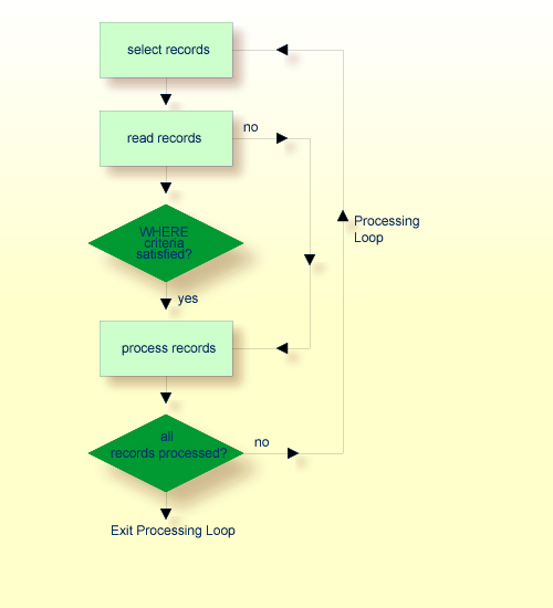
The following diagram illustrates the flow logic of a database processing loop:
The use of multiple FIND and/or
READ statements creates
a hierarchy of processing loops, as shown in the following
example:
** Example 'FINDX04': FIND  (two FIND statements nested)
************************************************************************
DEFINE DATA LOCAL
1 PERSONVIEW VIEW OF EMPLOYEES
  2 PERSONNEL-ID
  2 NAME
1 AUTOVIEW VIEW OF VEHICLES
  2 PERSONNEL-ID
  2 MAKE
  2 MODEL
END-DEFINE
*
EMP. FIND PERSONVIEW WITH NAME = 'ADKINSON'
  VEH. FIND AUTOVIEW WITH PERSONNEL-ID = PERSONNEL-ID (EMP.)
    DISPLAY NAME MAKE MODEL
  END-FIND
END-FIND
END
The above program selects from the EMPLOYEES file
all people with the name ADKINSON. Each record (person) selected
is then processed as follows:
The second FIND statement is executed to select
the automobiles from the VEHICLES file, using as selection
criterion the PERSONNEL-IDs from the records selected from the
EMPLOYEES file with the first FIND statement.
The NAME of each person selected is displayed;
this information is obtained from the EMPLOYEES file. The
MAKE and MODEL of each automobile owned by that
person is also displayed; this information is obtained from the
VEHICLES file.
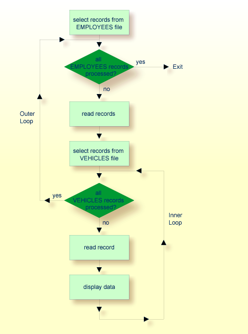
The second FIND statement creates an inner
processing loop within the outer processing loop of the first FIND
statement, as shown in the following diagram.
The diagram illustrates the flow logic of the hierarchy of processing loops in the previous example program:
It is also possible to construct a processing loop hierarchy in which the same file is used at both levels of the hierarchy:
** Example 'FINDX05': FIND (two FIND statements on same file nested)
************************************************************************
DEFINE DATA LOCAL
1 PERSONVIEW VIEW OF EMPLOYEES
  2 NAME
  2 FIRST-NAME
  2 CITY
1 #NAME (A40)
END-DEFINE
*
WRITE TITLE LEFT JUSTIFIED
  'PEOPLE IN SAME CITY AS:' #NAME / 'CITY:' CITY SKIP 1
*
FIND PERSONVIEW WITH NAME = 'JONES'
                WHERE FIRST-NAME = 'LAUREL'
  COMPRESS NAME FIRST-NAME INTO #NAME
  /*
  FIND PERSONVIEW WITH CITY = CITY
    DISPLAY NAME FIRST-NAME CITY
  END-FIND
END-FIND
END
The above program first selects all people with name
JONES and first name LAUREL from the
EMPLOYEES file. Then all who live in the same city are selected
from the EMPLOYEES file and a list of these people is created. All
field values displayed by the DISPLAY statement are taken from the
second FIND statement.
Output of Program FINDX05:
PEOPLE IN SAME CITY AS: JONES LAUREL
CITY: BALTIMORE

        NAME              FIRST-NAME              CITY
-------------------- -------------------- --------------------

JENSON               MARTHA               BALTIMORE
LAWLER               EDDIE                BALTIMORE
FORREST              CLARA                BALTIMORE
ALEXANDER            GIL                  BALTIMORE
NEEDHAM              SUNNY                BALTIMORE
ZINN                 CARLOS               BALTIMORE
JONES                LAUREL               BALTIMORE
See the following example programs:
This section describes how Natural performs database updating operations based on transactions.
The following topics are covered:
Natural performs database updating operations based on transactions, which means that all database update requests are processed in logical transaction units. A logical transaction is the smallest unit of work (as defined by you) which must be performed in its entirety to ensure that the information contained in the database is logically consistent.
A logical transaction may consist of one or more update statements
(DELETE,
STORE,
UPDATE) involving one
or more database files. A logical transaction may also span multiple Natural
programs.
A logical transaction begins when a record is put on
"hold"; Natural does this automatically when the record is read
for updating, for example, if a FIND loop contains an
UPDATE or DELETE statement.
The end of a logical transaction is determined by an
END TRANSACTION
statement in the program. This statement ensures that all updates within the
transaction have been successfully applied, and releases all records that were
put on "hold" during the transaction.
DEFINE DATA LOCAL
1 MYVIEW VIEW OF EMPLOYEES
  2 NAME
END-DEFINE
FIND MYVIEW WITH NAME = 'SMITH'
   DELETE
   END TRANSACTION
END-FIND
END
Each record selected would be put on "hold", deleted,
and then - when the END
TRANSACTION statement is executed - released from
"hold".
Note:
The Natural profile parameter
ETEOP, as
set by the Natural administrator, determines whether or not Natural will
generate an END TRANSACTION statement at the end of each Natural
program. Ask your Natural administrator for details.
The following example program adds new records to the
EMPLOYEES file.
** Example 'STOREX01': STORE (Add new records to EMPLOYEES file)
*
** CAUTION: Executing this example will modify the database records!
************************************************************************
DEFINE DATA LOCAL
1 EMPLOYEE-VIEW VIEW OF EMPLOYEES
2 PERSONNEL-ID(A8)
2 NAME (A20)
2 FIRST-NAME (A20)
2 MIDDLE-I (A1)
2 SALARY (P9/2)
2 MAR-STAT (A1)
2 BIRTH (D)
2 CITY (A20)
2 COUNTRY (A3)
*
1 #PERSONNEL-ID (A8)
1 #NAME (A20)
1 #FIRST-NAME (A20)
1 #INITIAL (A1)
1 #MAR-STAT (A1)
1 #SALARY (N9)
1 #BIRTH (A8)
1 #CITY (A20)
1 #COUNTRY (A3)
1 #CONF (A1) INIT <'Y'>
END-DEFINE
*
REPEAT
INPUT 'ENTER A PERSONNEL ID AND NAME (OR ''END'' TO END)' //
'PERSONNEL-ID : ' #PERSONNEL-ID //
'NAME : ' #NAME /
'FIRST-NAME : ' #FIRST-NAME
/*********************************************************************
/* validate entered data
/*********************************************************************
IF #PERSONNEL-ID = 'END' OR #NAME = 'END'
STOP
END-IF
IF #NAME = ' '
REINPUT WITH TEXT 'ENTER A LAST-NAME'
MARK 2 AND SOUND ALARM
END-IF
IF #FIRST-NAME = ' '
REINPUT WITH TEXT 'ENTER A FIRST-NAME'
MARK 3 AND SOUND ALARM
END-IF
/*********************************************************************
/* ensure person is not already on file
/*********************************************************************
FIP2. FIND NUMBER EMPLOYEE-VIEW WITH PERSONNEL-ID = #PERSONNEL-ID
/*
IF *NUMBER (FIP2.) > 0
REINPUT 'PERSON WITH SAME PERSONNEL-ID ALREADY EXISTS'
MARK 1 AND SOUND ALARM
END-IF
/*********************************************************************
/* get further information
/*********************************************************************
INPUT
'ENTER EMPLOYEE DATA' ////
'PERSONNEL-ID :' #PERSONNEL-ID (AD=IO) /
'NAME :' #NAME (AD=IO) /
'FIRST-NAME :' #FIRST-NAME (AD=IO) ///
'INITIAL :' #INITIAL /
'ANNUAL SALARY :' #SALARY /
'MARITAL STATUS :' #MAR-STAT /
'DATE OF BIRTH (YYYYMMDD) :' #BIRTH /
'CITY :' #CITY /
'COUNTRY (3 CHARS) :' #COUNTRY //
'ADD THIS RECORD (Y/N) :' #CONF (AD=M)
/*********************************************************************
/* ENSURE REQUIRED FIELDS CONTAIN VALID DATA
/*********************************************************************
IF #SALARY < 10000
REINPUT TEXT 'ENTER A PROPER ANNUAL SALARY' MARK 2
END-IF
IF NOT (#MAR-STAT = 'S' OR = 'M' OR = 'D' OR = 'W')
REINPUT TEXT 'ENTER VALID MARITAL STATUS S=SINGLE ' -
'M=MARRIED D=DIVORCED W=WIDOWED' MARK 3
END-IF
IF NOT(#BIRTH = MASK(YYYYMMDD) AND #BIRTH = MASK(1582-2699))
REINPUT TEXT 'ENTER CORRECT DATE' MARK 4
END-IF
IF #CITY = ' '
REINPUT TEXT 'ENTER A CITY NAME' MARK 5
END-IF
IF #COUNTRY = ' '
REINPUT TEXT 'ENTER A COUNTRY CODE' MARK 6
END-IF
IF NOT (#CONF = 'N' OR= 'Y')
REINPUT TEXT 'ENTER Y (YES) OR N (NO)' MARK 7
END-IF
IF #CONF = 'N'
ESCAPE TOP
END-IF
/*********************************************************************
/* add the record with STORE
/*********************************************************************
MOVE #PERSONNEL-ID TO EMPLOYEE-VIEW.PERSONNEL-ID
MOVE #NAME TO EMPLOYEE-VIEW.NAME
MOVE #FIRST-NAME TO EMPLOYEE-VIEW.FIRST-NAME
MOVE #INITIAL TO EMPLOYEE-VIEW.MIDDLE-I
MOVE #SALARY TO EMPLOYEE-VIEW.SALARY (1)
MOVE #MAR-STAT TO EMPLOYEE-VIEW.MAR-STAT
MOVE EDITED #BIRTH TO EMPLOYEE-VIEW.BIRTH (EM=YYYYMMDD)
MOVE #CITY TO EMPLOYEE-VIEW.CITY
MOVE #COUNTRY TO EMPLOYEE-VIEW.COUNTRY
/*
STP3. STORE RECORD IN FILE EMPLOYEE-VIEW
/*
/*********************************************************************
/* mark end of logical transaction
/*********************************************************************
END OF TRANSACTION
RESET INITIAL #CONF
END-REPEAT
END
Output of Program STOREX01:
ENTER A PERSONNEL ID AND NAME (OR 'END' TO END) PERSONNEL ID : NAME : FIRST NAME :
If Natural is used with Adabas, any record which is to be updated
will be placed in "hold" status until an
END TRANSACTION or
BACKOUT TRANSACTION
statement is issued or the transaction time limit is exceeded.
When a record is placed in "hold" status for one user, the record is not available for update by another user. Another user who wishes to update the same record will be placed in "wait" status until the record is released from "hold" when the first user ends or backs out his/her transaction.
To prevent users from being placed in wait status, the session
parameter WH
(Wait for Record in Hold Status) can be used (see the Parameter
Reference).
When you use update logic in a program, you should consider the following:
The maximum time that a record can be in hold status is
determined by the Adabas transaction time limit (Adabas parameter
TT). If this time limit is exceeded, you will receive an
error message and all database modifications done since the last
END TRANSACTION will
be made undone.
The number of records on hold and the transaction time limit
are affected by the size of a transaction, that is, by the placement of the
END TRANSACTION statement in the program. Restart facilities
should be considered when deciding where to issue an END
TRANSACTION. For example, if a majority of records being processed are
not to be updated, the GET statement is an efficient way
of controlling the "holding" of records. This avoids issuing
multiple END TRANSACTION statements and reduces the number of ISNs
on hold. When you process large files, you should bear in mind that the
GET statement requires an additional Adabas call. An example of a
GET statement is shown below.
The placing of records in "hold" status is also
controlled by the profile parameter RI (Release ISNs), as
set by the Natural administrator.
** Example 'GETX01': GET (put single record in hold with UPDATE stmt)
**
** CAUTION: Executing this example will modify the database records!
***********************************************************************
DEFINE DATA LOCAL
1 EMPLOY-VIEW VIEW OF EMPLOYEES
  2 NAME
  2 SALARY (1)
END-DEFINE
*
RD. READ EMPLOY-VIEW BY NAME
  DISPLAY EMPLOY-VIEW
  IF SALARY (1) > 1500000
    /*
    GE. GET EMPLOY-VIEW *ISN (RD.)
    /*
    WRITE '=' (50) 'RECORD IN HOLD:' *ISN(RD.)
    COMPUTE SALARY (1) = SALARY (1) * 1.15
    UPDATE (GE.)
    END TRANSACTION
  END-IF
END-READ
END
During an active logical transaction, that is, before the
END
                        				TRANSACTION
statement is issued, you can cancel the transaction by using a
BACKOUT TRANSACTION
statement. The execution of this statement removes all updates that have been
applied (including all records that have been added or deleted) and releases
all records held by the transaction.
With the END
TRANSACTION statement, you can also store transaction-related
information. If processing of the transaction terminates abnormally, you can
read this information with a GET
TRANSACTION DATA statement to ascertain where to resume
processing when you restart the transaction.
The following program updates the EMPLOYEES and
VEHICLES files. After a restart operation, the user is informed of
the last EMPLOYEES record successfully processed. The user can
resume processing from that EMPLOYEES record. It would also be
possible to set up the restart transaction message to include the last
VEHICLES record successfully updated before the restart
operation.
** Example 'GETTRX01': GET TRANSACTION
*
** CAUTION: Executing this example will modify the database records!
************************************************************************
DEFINE DATA LOCAL
01 PERSON VIEW OF EMPLOYEES
02 PERSONNEL-ID (A8)
02 NAME (A20)
02 FIRST-NAME (A20)
02 MIDDLE-I (A1)
02 CITY (A20)
01 AUTO VIEW OF VEHICLES
02 PERSONNEL-ID (A8)
02 MAKE (A20)
02 MODEL (A20)
*
01 ET-DATA
02 #APPL-ID (A8) INIT <' '>
02 #USER-ID (A8)
02 #PROGRAM (A8)
02 #DATE (A10)
02 #TIME (A8)
02 #PERSONNEL-NUMBER (A8)
END-DEFINE
*
GET TRANSACTION DATA #APPL-ID #USER-ID #PROGRAM
#DATE #TIME #PERSONNEL-NUMBER
*
IF #APPL-ID NOT = 'NORMAL' /* if last execution ended abnormally
AND #APPL-ID NOT = ' '
INPUT (AD=OIL)
// 20T '*** LAST SUCCESSFUL TRANSACTION ***' (I)
/ 20T '***********************************'
/// 25T 'APPLICATION:' #APPL-ID
/ 32T 'USER:' #USER-ID
/ 29T 'PROGRAM:' #PROGRAM
/ 24T 'COMPLETED ON:' #DATE 'AT' #TIME
/ 20T 'PERSONNEL NUMBER:' #PERSONNEL-NUMBER
END-IF
*
REPEAT
/*
INPUT (AD=MIL) // 20T 'ENTER PERSONNEL NUMBER:' #PERSONNEL-NUMBER
/*
IF #PERSONNEL-NUMBER = '99999999'
ESCAPE BOTTOM
END-IF
/*
FIND1. FIND PERSON WITH PERSONNEL-ID = #PERSONNEL-NUMBER
IF NO RECORDS FOUND
REINPUT 'SPECIFIED NUMBER DOES NOT EXIST; ENTER ANOTHER ONE.'
END-NOREC
FIND2. FIND AUTO WITH PERSONNEL-ID = #PERSONNEL-NUMBER
IF NO RECORDS FOUND
WRITE 'PERSON DOES NOT OWN ANY CARS'
ESCAPE BOTTOM
END-NOREC
IF *COUNTER (FIND2.) = 1 /* first pass through the loop
INPUT (AD=M)
/ 20T 'EMPLOYEES/AUTOMOBILE DETAILS' (I)
/ 20T '----------------------------'
/// 20T 'NUMBER:' PERSONNEL-ID (AD=O)
/ 22T 'NAME:' NAME ' ' FIRST-NAME ' ' MIDDLE-I
/ 22T 'CITY:' CITY
/ 22T 'MAKE:' MAKE
/ 21T 'MODEL:' MODEL
UPDATE (FIND1.) /* update the EMPLOYEES file
ELSE /* subsequent passes through the loop
INPUT NO ERASE (AD=M IP=OFF) //////// 28T MAKE / 28T MODEL
END-IF
/*
UPDATE (FIND2.) /* update the VEHICLES file
/*
MOVE *APPLIC-ID TO #APPL-ID
MOVE *INIT-USER TO #USER-ID
MOVE *PROGRAM TO #PROGRAM
MOVE *DAT4E TO #DATE
MOVE *TIME TO #TIME
/*
END TRANSACTION #APPL-ID #USER-ID #PROGRAM
#DATE #TIME #PERSONNEL-NUMBER
/*
END-FIND /* for VEHICLES (FIND2.)
END-FIND /* for EMPLOYEES (FIND1.)
END-REPEAT /* for REPEAT
*
STOP /* Simulate abnormal transaction end
END TRANSACTION 'NORMAL '
END
This section discusses the statements ACCEPT and
REJECT which are used to select records based on user-specified
logical criteria.
The following topics are covered:
The statements ACCEPT and
REJECT can be used in
conjunction with the database access statements:
** Example 'ACCEPX01': ACCEPT IF
************************************************************************
DEFINE DATA LOCAL
1 MYVIEW VIEW OF EMPLOYEES
  2 NAME
  2 JOB-TITLE
  2 CURR-CODE (1:1)
  2 SALARY    (1:1)
END-DEFINE
*
READ (20) MYVIEW BY NAME WHERE CURR-CODE (1) = 'USD'
ACCEPT IF SALARY (1) >= 40000
  DISPLAY NAME JOB-TITLE SALARY (1)
END-READ
END
Output of Program ACCEPX01:
   Page      1                                                  04-11-11  11:11:11

          NAME                  CURRENT            ANNUAL
                               POSITION            SALARY
  -------------------- ------------------------- ----------

  ADKINSON             DBA                            46700
  ADKINSON             MANAGER                        47000
  ADKINSON             MANAGER                        47000
  AFANASSIEV           DBA                            42800
  ALEXANDER            DIRECTOR                       48000
  ANDERSON             MANAGER                        50000
  ATHERTON             ANALYST                        43000
  ATHERTON             MANAGER                        40000
The statements ACCEPT and
REJECT allow you to
specify logical conditions in addition to those that were specified in
WITH and
WHERE clauses
of the READ
statement.
The logical condition criteria in the IF clause of an
ACCEPT /
REJECT statement are
evaluated after the record has been selected and read.
Logical condition operators include the following (see Logical Condition Criteria for more detailed information):
EQUAL |
EQ |
:= |
NOT EQUAL TO |
NE |
¬= |
LESS THAN |
LT |
< |
LESS EQUAL |
LE |
<= |
GREATER THAN |
GT |
> |
GREATER EQUAL |
GE |
>= |
Logical condition criteria in ACCEPT /
REJECT statements may
also be connected with the Boolean operators AND, OR,
and NOT. Moreover, parentheses may be used to indicate logical
grouping; see the following examples.
The following program illustrates the use of the Boolean operator
AND in an ACCEPT statement.
** Example 'ACCEPX02': ACCEPT IF ... AND ...
************************************************************************
DEFINE DATA LOCAL
1 MYVIEW VIEW OF EMPLOYEES
  2 NAME
  2 JOB-TITLE
  2 CURR-CODE (1:1)
  2 SALARY    (1:1)
END-DEFINE
*
READ (20) MYVIEW BY NAME WHERE CURR-CODE (1) = 'USD'
ACCEPT IF  SALARY (1) >= 40000
         AND SALARY (1) <= 45000
  DISPLAY NAME JOB-TITLE SALARY (1)
END-READ
END
Output of Program ACCEPX02:
Page      1                                                  04-12-14  12:22:01

        NAME                  CURRENT            ANNUAL
                             POSITION            SALARY
-------------------- ------------------------- ----------

AFANASSIEV           DBA                            42800
ATHERTON             ANALYST                        43000
ATHERTON             MANAGER                        40000
The following program, which uses the Boolean operator
OR in a REJECT statement, produces the
same output as the ACCEPT statement in the example above, as the
logical operators are reversed.
** Example 'ACCEPX03': REJECT IF ... OR ...
************************************************************************
DEFINE DATA LOCAL
1 MYVIEW VIEW OF EMPLOYEES
  2 NAME
  2 JOB-TITLE
  2 CURR-CODE (1:1)
  2 SALARY    (1:1)
END-DEFINE
*
READ (20) MYVIEW BY NAME WHERE CURR-CODE (1) = 'USD'
REJECT IF SALARY (1) < 40000
         OR SALARY (1) > 45000
  DISPLAY NAME JOB-TITLE SALARY (1)
END-READ
END
Output of Program ACCEPX03:
Page      1                                                  04-12-14  12:26:27

        NAME                  CURRENT            ANNUAL
                             POSITION            SALARY
-------------------- ------------------------- ----------

AFANASSIEV           DBA                            42800
ATHERTON             ANALYST                        43000
ATHERTON             MANAGER                        40000
See the following example programs:
This section discusses the use of the statements AT START
OF DATA and AT END OF DATA.
The following topics are covered:
The AT START OF
DATA statement is used to specify any processing that is to
be performed after the first of a set of records has been read in a database
processing loop.
The AT START OF DATA statement must be placed within
the processing loop.
If the AT START OF DATA processing produces any
output, this will be output before the first field value. By default,
this output is displayed left-justified on the page.
The AT END OF
DATA statement is used to specify processing that is to be
performed after all records for a database processing loop have been
processed.
The AT END OF DATA statement must be placed within
the processing loop.
If the AT END OF DATA processing produces any output,
this will be output after the last field value. By default, this
output is displayed left-justified on the page.
The following example program illustrates the use of the
statements AT START OF DATA and AT END OF DATA.
The Natural system variable
*TIME
has been incorporated into the AT START OF DATA statement to
display the time of day.
The Natural system function OLD has been incorporated
into the AT END OF DATA statement to display the name of the last
person selected.
** Example 'ATSTAX01': AT START OF DATA
************************************************************************
DEFINE DATA LOCAL
1 MYVIEW VIEW OF EMPLOYEES
2 CITY
2 NAME
2 JOB-TITLE
2 INCOME (1:1)
3 CURR-CODE
3 SALARY
3 BONUS (1:1)
END-DEFINE
*
WRITE TITLE 'XYZ EMPLOYEE ANNUAL SALARY AND BONUS REPORT' /
READ (3) MYVIEW BY CITY STARTING FROM 'E'
DISPLAY GIVE SYSTEM FUNCTIONS
NAME (AL=15) JOB-TITLE (AL=15) INCOME (1)
/*
AT START
                     			 OF DATA
WRITE 'RUN TIME:' *TIME /
END-START
AT END OF
                        				DATA
WRITE / 'LAST PERSON SELECTED:' OLD (NAME) /
END-ENDDATA
END-READ
*
AT END OF PAGE
WRITE / 'AVERAGE SALARY:' AVER (SALARY(1))
END-ENDPAGE
END
The program produces the following output:
                  XYZ EMPLOYEE ANNUAL SALARY AND BONUS REPORT

     NAME           CURRENT                 INCOME
                   POSITION
                                CURRENCY   ANNUAL     BONUS
                                  CODE     SALARY
--------------- --------------- -------- ---------- ----------

RUN TIME: 12:43:19.1

DUYVERMAN       PROGRAMMER      USD           34000          0
PRATT           SALES PERSON    USD           38000       9000
MARKUSH         TRAINEE         USD           22000          0

LAST PERSON SELECTED: MARKUSH


AVERAGE SALARY:      31333
See the following example programs:
Natural enables users to access wide-character fields (format W) in an Adabas database.
The following topics are covered:
Adabas wide-character fields (W) are mapped to Natural format U (Unicode).
The length definition for a Natural field of format U corresponds
to half the size of the Adabas field of format W. An Adabas wide-character
field of length 200 is, for example, mapped to (U100)
in Natural.
Natural receives data from Adabas and sends data to Adabas using UTF-16 as common encoding.
This encoding is specified with the
OPRB
parameter and sent to Adabas with the open request. It is used for
wide-character fields and applies to the entire Adabas user session.
Collating descriptors are not supported.
For further information on Adabas and Unicode support refer to the specific Adabas product documentation.