MashZone is a browser-based application from Software AG which is used to visualize data on a graphical, interactive dashboard, a so-called MashApp. The Natural Profiler MashApps evaluate the Profiler event data and depict it in MashZone.
This document covers the following topics:
This section provides instructions for implementing the MashApps:
The Natural Profiler MashApps and related data are supplied as a Natural component in a zip file.
![]() To download the MashApps zip file
To download the MashApps zip file
Log in to Software AG's Empower web site at https://empower.softwareag.com/ (password required).
Go to Products & Documentation > Download Components.
The Download Components section is displayed.
From the Download Components section, select Natural Profiler MashApp.
Download the NaturalProfiler_MashApp.zip file.
In addition to the zip file, Empower also provides the Readme file
Readme_ NaturalProfiler_MashApp.txt which contains the latest
update information.
You have to unpack the MashApp zip file in the appropriate MashZone directory which depends on the MashZone version installed at your site.
![]() To unpack the MashApp zip file
To unpack the MashApp zip file
Unpack the NaturalProfiler_MashApp.zip file in the
appropriate user data directory of MashZone:
For MashZone Version 9.0 and above:
installation-directory\server\bin\work\work_mashzone_server-type\mashzone_data
where server-type
indicates the type of the MashZone server: s, m or
i. For example, work_mashzone_m for a medium type.
For MashZone versions below Version 9.0:
installation-directory
where
installation-directory is the MashZone
installation directory.
After unpacking the zip file, the following subdirectories are available in the user data directory of MashZone:
| Directory | Content |
|---|---|
importexport\Profiler_date |
MashApps for the Natural Profiler.
|
resources\Profiler |
Parent directory of Profiler resources.
Contains the user-modified See also Editing the Overview.csv Resource File. |
resources\Profiler\Definition |
Resources used by the MashApp.
Initially, this directory contains the resources which do not have to be edited. |
resources\Profiler\Data |
Profiler data directory (including subdirectories) in which the Profiler data files are stored by default. |
resources\Profiler_src |
Source directory for resources which have to
be edited and copied into the resources\Profiler directory.
See also Editing the Overview.csv Resource File. |
assets\colorschemes |
Color schemes.
The color schemes for the Natural Profiler are named
|
You can edit the Overview.csv resource file in the
resources\Profiler_src directory to adapt the Natural Profiler
MashApps to your requirements. The resource file is a CSV-formatted file with
semicolon (;) separators which can be edited with any text editor.
The supplied Overview.csv file contains one line for the
sample Profiler data in the Profiler_Sample.csv file in the
resources\Profiler\Data directory. Add more lines for each
Profiler CSV file you want to evaluate. For information on creating Profiler
CSV files, see Preparing the Profiler
Data. You can also add or delete lines in the
Overview.csv file later, after you have copied it to the
resources\Profiler directory (see
Activating the
MashApp).
In the columns of the Overview.csv, you can specify the
following:
| Column | Description |
|---|---|
csv File |
Specify the name of the Profiler consolidated
data file.
If the data file resides in a subdirectory of
Specify |
Description |
Specify a descriptive name for the Profiler
consolidated data file. The descriptions are used in the
Input selection box of the Natural Profiler MashApps.
If you do not enter a value, the value of the csv File column is used in the Input selection box. |
Enable |
If you enter Y in this column, the
name or description of the Profiler consolidated data file is shown in the
Input selection box. Otherwise, it is not shown.
|
Prerequisites for activating the Natural Profiler MashApps are a Professional, Enterprise or Event license file and administrator rights.
![]() To activate the MashApps
To activate the MashApps
Copy the resource file from resources\Profiler_src to
resources\Profiler.
Invoke MashZone.
Go to the Administration page (see the corresponding tab at the top of the page) and then to the Import/Export/Delete page.
Import the MashZone archive files (*.mzp) from the
importexport\Profiler_date directory by
using the Import function.
The MashApps in the
importexport\Profiler_date directory
are named as follows:
M_MashAppName
                                       version_revision_date-time.mzp
where MashAppName is the
name of the MashApp in MashZone which can be either of the following:
| MashAppName | Purpose |
|---|---|
Natural Profiler |
Evaluate the Natural Profiler data and the Profiler properties and statistics of a monitored application. |
Natural Profiler Compare |
Compare two Natural Profiler data files. |
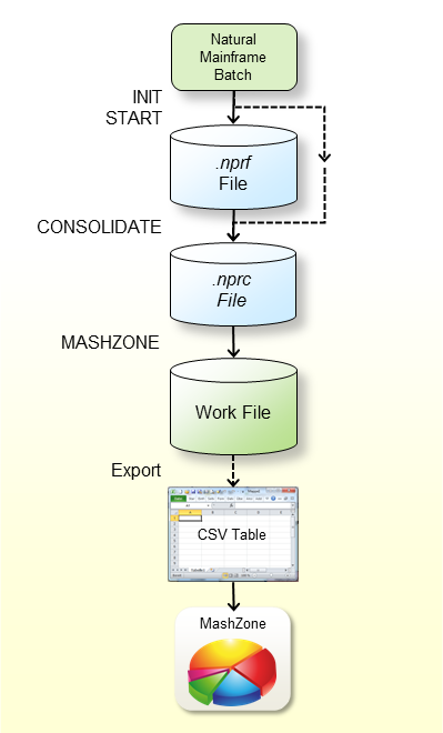
The graphic above illustrates the steps you have to perform before you can evaluate the Natural Profiler data in MashZone:
Profile the Natural mainframe batch application with the Natural
Profiler data collection functions as described in the section
Using the Profiler Utility in
Batch Mode. The Profiler writes the event data to an
.nprf Natural Profiler resource file.
Consolidate the event data using the Profiler utility
CONSOLIDATE
function. The consolidated data is written to an .nprc Natural
Profiler resource consolidated file.
Alternatively, you can specify CONSOLIDATE=ON with the
Profiler utility INIT function when you profile the Natural
mainframe batch application. In this case, the Profiler writes the event data
directly to an .nprc Natural Profiler resource file.
Write the consolidated event data with the Profiler utility
MASHZONE function
in CSV (comma-separated values) format to Work File 7.
Export the data from Work File 7 with any tool (such as FTP) to the
Profiler data directory (see Unpacking the Zip
File). Use .csv as the file extension.
Enter a reference to the new file in the Overview.csv
file in the resources\Profiler directory.
If you start MashZone, you will find the description of the new file in the Input selection box. If you select the line with the description, the Natural Profiler MashApps read the event data from the corresponding CSV file.
If you already started the Natural Profiler MashApp earlier, MashZone
may not immediately detect the new entry in the Overview.csv file.
In this case, start any other MashApp, and then restart the Natural Profiler
MashApp to clear the internal MashZone buffer.
After you have specified all required information as described in the previous sections, you can proceed as follows:
Invoke MashZone.
Open the Natural Profiler MashApp or the Natural Profiler Compare MashApp.
The Natural Profiler MashApp offers two tabbed pages for analyzing the Profiler event data and viewing the Profiler properties and statistics:
The Evaluation page provides the Profiler event data evaluation.
The Properties page lists the Profiler properties and the statistics of the monitored application.
The Natural Profiler Compare MashApp offers two tabbed pages for comparing the Profiler event data and the Profiler properties and statistics:
The Compare page compares the Profiler event data of two monitored applications.
The Properties page lists the Profiler properties and the statistics of the two monitored applications.
The pages are described in the following section.
The Evaluation page (Natural Profiler MashApp) looks similar to the example below:
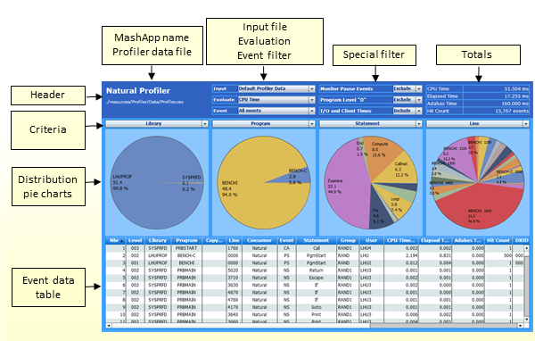
The Evaluation page is organized in the following sections:
The header at the top of the page with Input and KPI selection fields, filters and totals;
The selection boxes for the distribution criteria and corresponding distribution pie charts;
The event data table at the bottom of the page with the consolidated event data.
This section covers the following topics:
The header contains the following elements (from left to right and top to bottom):
The name of the MashApp.
The path and name of the Profiler data file currently selected.
The Input selection box which is used to select
the Profiler data file. The file names listed for selection are taken from the
Description column in the Overview.csv file. See
Editing the Overview.csv
Resource File. The selected file is used for both pages of
the Natural Profiler MashApp.
The Evaluate selection box which is used to select the KPI you want to evaluate in the pie charts. The following KPIs are available:
CPU Time
Elapsed Time
Adabas Command Time
Hit Count
The CPU time is evaluated by default. All time values are expressed in milliseconds.
The Event selection box is used to filter the event type you want to evaluate. The event types available for selection depend on the event types collected with the Natural Profiler. The pie charts, the event data table and the totals reflect only the data returned for the selected event types. By default, all event types are evaluated.
Filtering specific event types is especially useful, for example, to evaluate the hit count of events that seldom occur such as error events.
The Monitor Pause Events selection box is used to filter Monitor Pause events. The filter is valid for the pie charts, the event data table and the totals. By default, the evaluations do not reflect Monitor Pause events. If you include Monitor Pause events, you can see how often monitoring paused, and how long and why it paused.
The Program Level “0” selection box is used to
filter events which are executed at Program Level 0. These events
usually relate to the Natural administration rather than the application
execution. The filter is valid for the pie charts, the event data table and the
totals. By default, the evaluations do not reflect the events at the program
level 0.
The I/O and Client Times selection box is used
to filter the I/O time (IB event) and the Natural RPC client time
(RW event). These times mainly measure the user reaction (how long
it took to press ENTER), especially when the elapsed time for an
interactive application is evaluated. They are less relevant for the
application performance. The filter is valid for the pie charts, the event data
table and the totals. By default, the evaluations reflect the I/O and client
times.
Summarized totals for the CPU time, the elapsed time, the Adabas time and the hit count according to the values that are currently selected in the header and in the pie charts.
The Evaluation page contains four pie charts. Each pie chart shows the distribution of the KPI (selected in the Evaluate selection box) for the criterion selected in the box directly above the pie chart (see the example in Evaluating Distribution Pie Charts).
This section covers the following topics:
The following criteria are available for all event types:
- Consumer
The consumer combines one or more event types into a new criterion. The new criterion depends on the process that consumed the CPU or elapsed time given with the event data. For example, the time returned for a Before Database Call (
DB) event is consumed by the database (and therefore belongs to the Database consumer), whereas the time returned for an After Database Call (DA) event is consumed by the Natural application (and therefore belongs to the Natural consumer).A consumer evaluation is not relevant for an Adabas time or hit count analysis.
The following consumers are provided:
Consumer Event Type Description Administration PL,PTThe time Natural used to load and release Natural objects. On the mainframe, the loading of Natural objects from the Natural system file is charged to the Database consumer (
DBevent against FNAT or FUSER system file).On UNIX and Windows, the entire operation is charged to the Administration consumer.
Database DBThe time consumed for database calls. For the CPU time, it is the time spent in the Natural region.
External CBThe time spent for external (non-Natural) program calls. I/O IBThe time spent for I/Os. When you analyze the elapsed time of an interactive application, this section shows the user response time.
This section is only displayed if I/O and Client Times is included in the selection box in the page header.
Pause MPThe time for which the monitor paused. This section is only displayed if Monitor Pause Events is included in the selection box in the page header.
RPC Client RWThe time spent on the Natural RPC client side. When you analyze the elapsed time of an interactive RPC application, this section shows the user’s response time.
This section is only displayed if I/O and Client Times is included in the selection box in the page header.
RPC Server RI,ROThe time consumed by the Natural RPC server layer. Session SI,STThe time required to initialize the Natural session. Natural CA,DA,E,IA,NS,PR,PS,RS,UThe time Natural spent executing the program code. - Event
The type of the event to be evaluated. All event types are listed in Events and Data Collected in the section Using the Profiler Utility in Batch Mode.
For technical reasons, a Program Resume (
PR) event uses the same timestamp as the Program Termination (PT) event that immediately precedes thePRevent. Therefore, thePTevent generally shows a CPU time and elapsed time of zero (0).- Group
The group ID for Natural RPC applications running under Natural Security.
- Level
The level at which the profiled program executes.
- Library
The Natural library that contains the profiled program.
- Line
The source line in which the Natural statement executed by the profiled program is coded.
- Line100
Source lines with similar line numbers (rounded down to the next multiple of 100).
- Program
The name of the profiled program.
- Statement
The Natural statement (for example,
EXAMINE) executed in the profiled program.- User
The user ID for Natural RPC applications running under Natural Security.
The following criteria are only available for specific event types. If you select an event-specific criterion, the pie chart will only reflect the data of the related events.
- Client User
The Natural RPC client user ID type for
RI,ROandRWevents.- Command
The Adabas command for
DBandDAevents.- File
The database ID and file number of the Natural system file for
PSandPTevents.
The database ID and file number of the Adabas file accessed forDBandDAevents.- Return Code
The termination return code for
STevents.
The database response and subcode forDAevents.
The subprogram response code forCAevents.
The error number forEevents.
The Natural RPC return code forRI,ROandRWevents.- Target Program
The session backend program name for
STevents.
The target program name forPLevents.
The name of the called subprogram forCBandCAevents.
The error handling program name forEevents.
The Natural RPC subprogram name forRSevents.- Type
The program type for
PSandPTevents.
The monitor pause reason forMPevents.
The user event subtype forUevents.
The return code indicator (system or user) forSTevents.
This section describes how you can evaluate distribution pie charts.
A distribution pie chart shows the distribution for the criterion currently selected in the selection box directly above the pie chart. In the following example, Statement has been selected as the criterion for evaluating the CPU time:
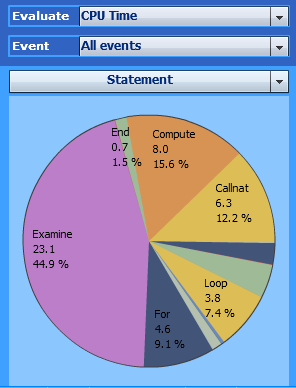
The pie chart shows the distribution of the CPU time for the used
Natural statements. It indicates that the Examine
statement consumed the most CPU time (23.1 ms / 44.9
percent).
If you click on a segment in the pie chart, all following pie charts, the event data table and the totals use the selected value as the filter criterion. In the example below, the Examine statement in the left pie chart has been selected:
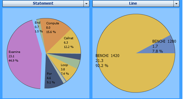
The right pie chart above displays only those two lines in which an Examine statement is executed. The event data table at the bottom of the page and the totals in the page header also reflect the data for the Examine statement only.
To remove a selection, click on the background of a pie chart.
If you move the cursor to the upper right corner of a pie chart, a drop down list provides the option to save the pie chart as a picture or to display and save the related data. For the display, a window opens with a table containing the data monitored for the Natural statements:
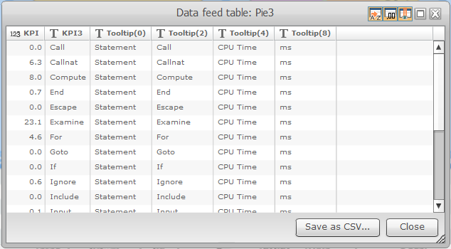
In the example above, the table lists the values of the left pie chart in the previous graphic. The KPI column lists the CPU time and the KPI3 column the corresponding Natural statement.
You can save the table data as a CSV (comma-separated values) formatted file.
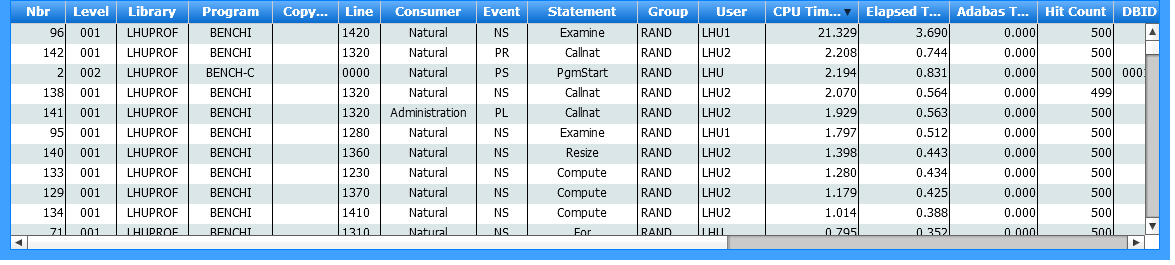
The event data table at the bottom of the Evaluation page lists the consolidated Profiler event data according to the values currently selected in the page header and the pie charts. If you click on the table header of a column, the data is sorted by that column.
In the following example, the event data table is sorted by the CPU time (descending):
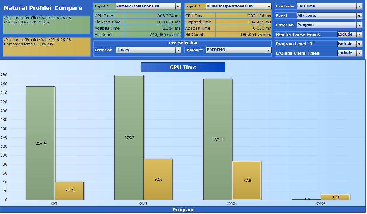
The Compare page (Natural Profiler Compare MashApp) compares the Profiler event data of two monitored applications as shown in the following example:
The Compare page is organized in the following sections:
The header at the top of the page with Input and KPI selection fields, filters and totals.
The column chart comparing the values of the two monitored applications:
Values for the first application are shown in the left (green) column, values for the second application are shown in the right (yellow) column.
This section covers the following topics:
The Compare header contains the following elements (from left to right and top to bottom):
The name of the MashApp.
The paths and names of the two Profiler data files to be compared.
The Input 1 and Input 2
selection boxes with the Profiler data files selected for comparison. The file
names listed for selection are taken from the Description column
in the Overview.csv file (see
Editing the Overview.csv
Resource File). The selected files are used for both pages
of the Natural Profiler Compare MashApp.
Summarized totals for the CPU time, the elapsed time, the Adabas time and the hit count according to the values for both applications listed in the header and column chart.
The Evaluate selection box with the KPI to evaluate in the column chart (see Evaluation Header).
The Event selection box with the event type to evaluate for (see Evaluation Header).
The Criterion selection box with the filter criterion to use for the KPI distribution. The criteria available for selection correspond to the criteria for the distribution pie charts on the Evaluation page (see Evaluating Distribution Pie Charts.
The Monitor Pause Events selection box with the filter criterion to use for Monitor Pause events (see Evaluation Header).
The Program Level "0" selection box with the
filter criterion to use for events at the program level 0 (see
Evaluation
Header).
The I/O and Client Times selection box with the
filter criterion to use for I/O time (IB event) and Natural RPC
client time (RW event) events; see
Evaluation
Header.
The Pre-Selection values with restrictions for the column chart values to a specific criterion instance, for example to a specific library.
The Compare column chart compares the values of the KPI (selected in the Evaluate selection box) for the criterion specified in the Criterion selection box for both profiled applications.
In the example of a Compare page
shown earlier, the CPU time (Evaluate selection box) of
each program (Criterion selection box) executed by
Numeric Operations MF (Input 1) is compared
with the corresponding time of Numeric Operations LUW
(Input 2). Additionally, a pre-selection has been
specified so that only values from the library PRFDEMO are
considered. The green columns show the CPU times of Numeric Operations
MF, the yellow columns the CPU times of Numeric Operations
LUW.
The Properties page lists the Profiler properties and the statistics of the monitored application as shown in the following example:
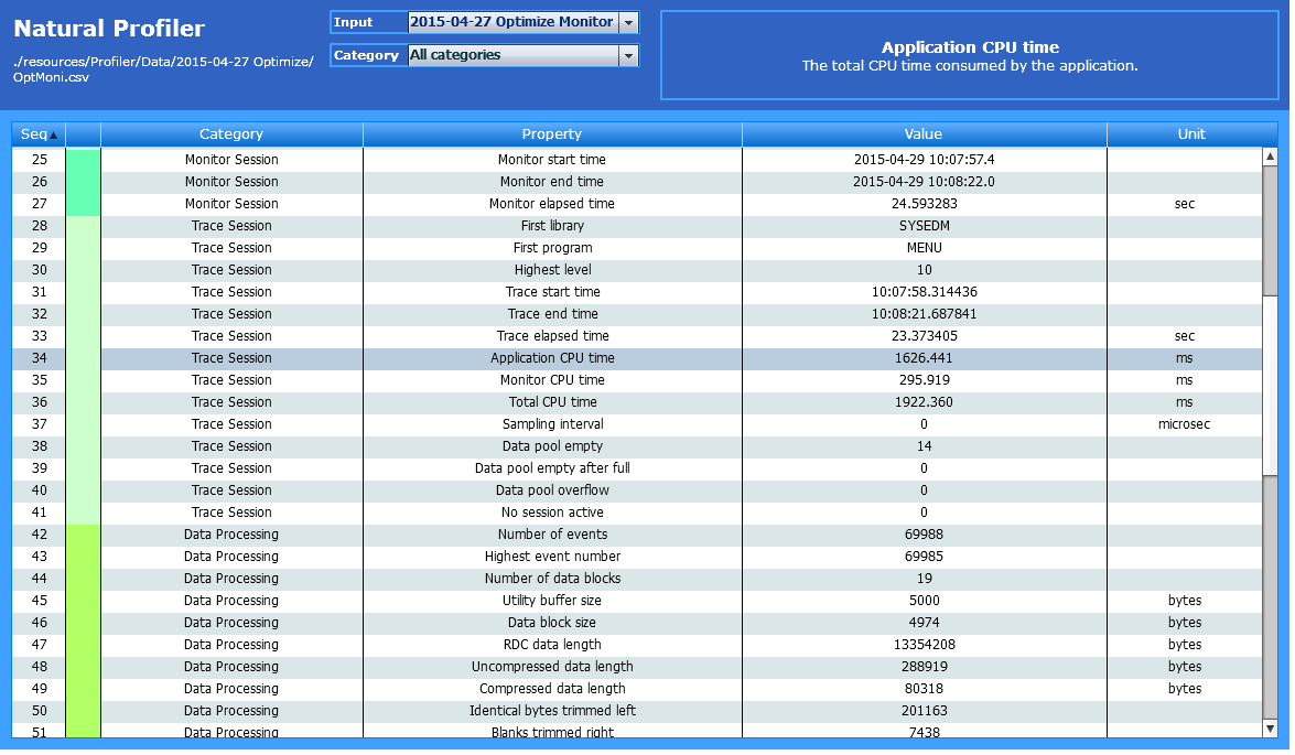
The Properties page of the Natural Profiler Compare MashApp lists the properties and statistics of both Profiler data files selected for comparison.
The Properties page is organized in the following sections:
The properties header at the top of the page with Input and Category selection fields and the property description;
The properties table with the properties and statistics.
This section covers the following topics:
The header contains the following elements (from left to right and top to bottom):
The name of the MashApp.
The path and name of the Profiler data file currently selected.
The Input selection box is used to select the
Profiler data file. The names listed for selection are taken from the
Description column in the Overview.csv file. See
Editing the Overview.csv
Resource File. The selected file is used for both pages of
the Natural Profiler MashApp.
The Category selection box is used to select a category (listed alphabetically). The selection box only offers the categories for which at least one associated property is found in the Profiler data file.
If you select a category, the table shows the properties of the selected category only. By default, all categories are displayed. The following categories are available:
| Category | Description |
|---|---|
| Data Consolidation | Statistics of the data consolidation such as the consolidation factor |
| Data Processing | Statistics of the data processing, data compression and data transfer such as the number of events and the compression rate |
| Event Type Statistics | Statistics of the event types such as the number of Program Load events |
| General Info | Information related to the environment and the Natural Profiler such as the internal Profiler version |
| Monitor Pause Statistics | Statistics of Monitor Pause events such as the number of Profiler data pool full situations |
| Monitor Session | Statistics of the Profiler monitor session such as the monitor elapsed time |
| Profiler Resource File | Information related to the Profiler resource file such as the resource name and library |
| Trace Session | Statistics of the Profiler trace session including the application execution such as the CPU time of the total session |
The Property description. If you click on a line in the properties table, the name of the corresponding property and a detailed description of it are displayed in the page header.
The properties table lists all collected Profiler properties and application statistics. If you click on an entry in the table header of a column, the entire table is sorted by this column. Each color in the second column corresponds to one category.
All Profiler categories and properties are described in detail in the section Profiler Statistics.
This section describes the following use cases:
By default, the Natural Profiler MashApp is set up to create CPU time performance analyses of libraries, programs, statements and source lines.
Each pie chart in the example below shows the distribution of the CPU time for each criterion selected:
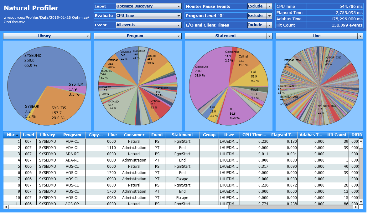
You can immediately see which library, program, statement or line has consumed how much of the CPU time.
The example above uses the following selections:
| Evaluate: | CPU Time |
| Event: | All events |
| Criteria: | Library, Program, Statement, Line |
A large application, such as the example above, references many program lines, thus making it difficult to analyze the corresponding pie chart.
If you click on a segment in a pie chart, the corresponding value of
that segment is used as a filter and the amount of data which is displayed in
the following pie charts is reduced accordingly. In the example above, a click
on the segment with the SYSEDMD library in the leftmost pie chart
would change the contents of the other three pie charts and only show the
programs, statements and lines executed in the SYSEDMD
library.
The following example refers to the previous one and assumes that in
addition to the SYSEDMD library, the program DISADA2,
the Callnat statement and the line 3564 are selected
in the rightmost chart:
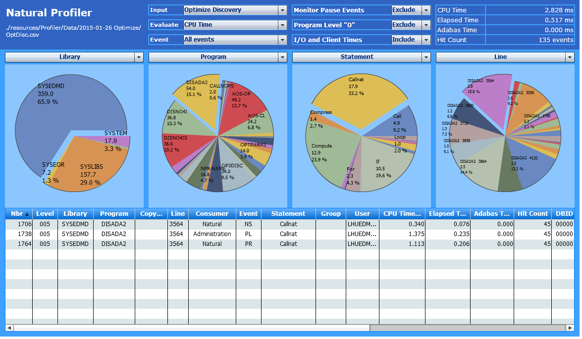
The event data table and the total in the page header now only refer to
Line 3564 where the program executes the CALLNAT statement. The
CALLNAT statement caused the event types (NS,
PL and PR), each executing 45 times
which results in a total Hit Count of 135
events.
The Line100 criterion is another approach to reduce the number of entries in the line number chart. It replaces the lines by the previous multiples of 100, thus, combining lines with similar line numbers in one segment of the pie chart.
The example below assumes that you want to find out which part of the
program OP3DISC consumed the most CPU time. Therefore, you select
OP3DISC in the Program chart so that all
other charts only display the data for this program:
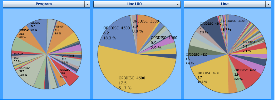
The Line chart clearly indicates that the
statement in the segment of line 4630 uses 19.9
percent of the program’s CPU time. However, all other segments are rather small
and it is difficult to tell them apart.
The Line100 chart shows that more than half of the time was consumed by the statements in the lines ranging from 4600 through 4690. Additionally, considering the statements in the lines ranging from 4500 through 4590, this part of the program even consumes 70 percent of the entire execution time. Thus, this program is most busy with the statements in these lines.
The example above uses the following selections:
| Evaluate: | CPU Time |
| Event: | All events |
| Criteria: | Program, Line, Line100 |
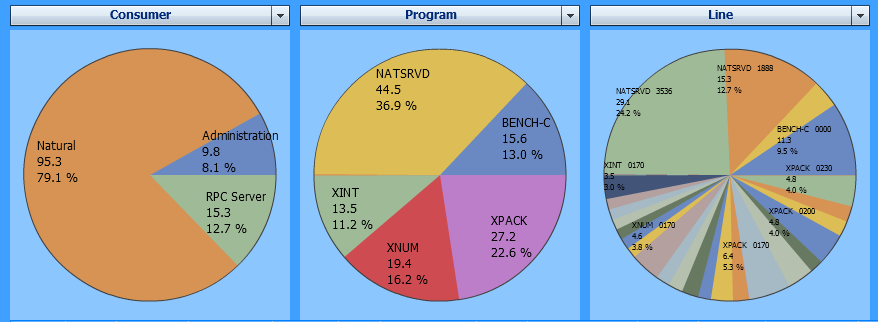
The Consumer analysis gives a quick overview of the processes that consumed the most CPU time such as external programs, database calls, I/Os, administration tasks or program instructions. For example:
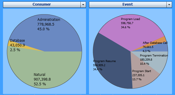
In the example above (Natural for UNIX, without statement events),
45 % of the CPU time was consumed by administration tasks. A
potential reason for this can be the usage of small subprograms which solely
call other tiny subprograms. This keeps Natural busy with administration tasks
(program load with buffer pool management and program termination), while the
time used for executing the code itself is relatively short.
The example above uses the following selections:
| Evaluate: | CPU Time |
| Event: | All events |
| Criteria: | Consumer, Event |
When analyzing the elapsed time of an interactive application, waiting
for a user response usually takes the most time. For a Natural RPC application,
this time is monitored with the RPC Wait for Client (RW) event or
the RPC Client consumer.
In the example below, the Natural RPC client consumes nearly all of the elapsed time:
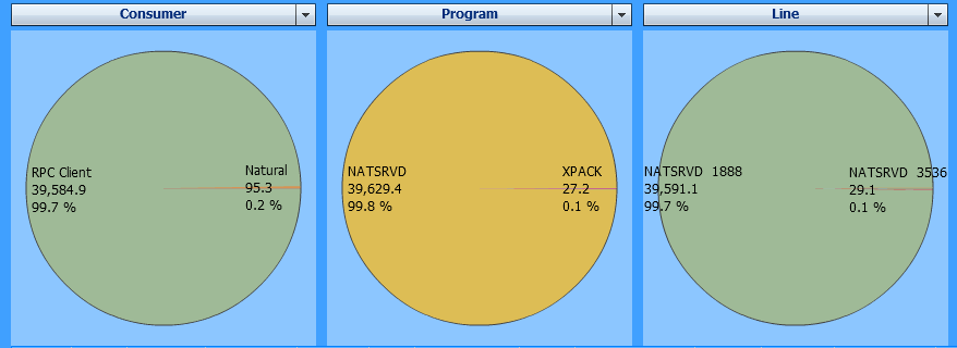
The example above uses the following selections:
| Evaluate: | Elapsed Time |
| Event: | All events |
| I/O and Client Times: | Include |
| Criteria: | Consumer, Program, Line |
The MashApp offers a selection field to exclude the client time. If you exclude I/O and Client Times, all individual processes performed in the server application are shown similar to the example below:
The example above uses the following selections:
| Evaluate: | Elapsed Time |
| Event: | All events |
| I/O and Client Times: | Exclude |
| Criteria: | Consumer, Program, Line |
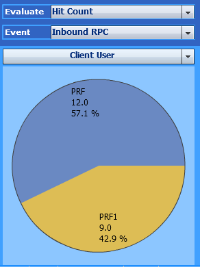
You can obtain statistics on remote procedure calls by evaluating the hit count.
- Example of a Natural RPC Client User Evaluation
The following example shows which user issued Natural RPC requests and how often:
In the example above, the user
PRFissued12Natural RPC requests.The example uses the following selections:
Evaluate: Hit Count Event: Inbound RPC Criterion: Client User - Example of a Natural RPC Target Program Evaluation
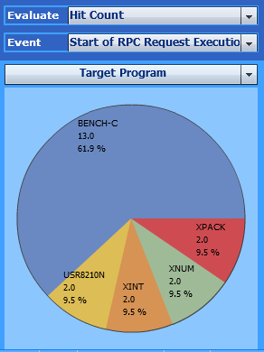
The following example displays which target program was called on the server and how often:
In the example above,
13Natural RPC requests were issued for the server programBENCH-C.The example uses the following selections:
Evaluate: Hit Count Event: Start of RPC Request Execution Criterion: Target Program
In both examples shown above, single event types are used for the event
selection so not to mix the data with other events. For example, if
All events is selected, the target programs of external
program calls (CA events) are also displayed in the chart.
When the Natural application issues an Adabas command, the database returns the elapsed time the Adabas nucleus required to process the command.
The example below analyzes the distribution of the Adabas command time for the accessed files and for the used Adabas commands. The chart also shows the programs and Natural statements that consumed the Adabas command time.
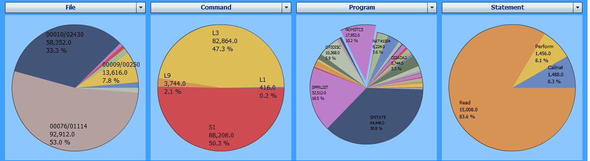
The most Adabas command time was consumed by calls against the file
1114 of the database 76 and by the Adabas commands
S1 (find record) and L3
(read logical sequential record).
If you could click on a segment in the pie chart below
File, you would see the commands issued against the
selected file and how much time they consumed. Since the segment of the program
NOMSTCS is selected in the third pie chart, the fourth pie chart
only shows the Adabas command time used by the statements in
NOMSTCS.
The example uses the following selections:
| Evaluate: | Adabas Command Time |
| Event: | All events |
| Criteria: | File, Command, Program, Statement |
You can obtain statistics on Adabas requests by evaluating the hit count.
The following example shows which files have been accessed, which commands have been issued, which Adabas response codes have occurred and which Natural statements have issued Adabas requests and how often:
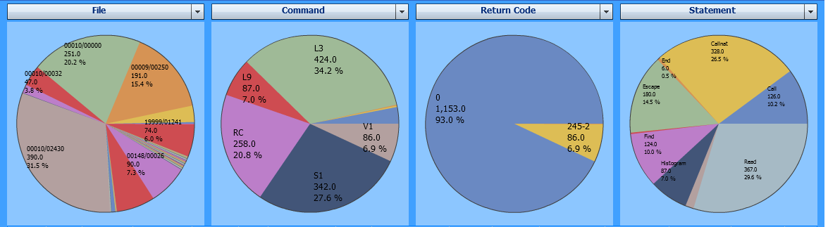
The most Adabas requests were issued against the file 2430
of database 10 and the most frequently Adabas command used was
L3 (read logical sequential record). Most calls were successful
(Adabas response 0) but 86 calls received an Adabas response
245 with subcode 2. The fourth pie chart shows that
READ statements issued 367 Adabas calls.
The example uses the following selections:
| Evaluate: | Hit Count |
| Event: | After Database Call |
| Criteria: | File, Command, Return Code, Statement |
The following Profiler MashApp examples may answer common statistics questions about monitored Natural applications.
Use the following selections to find out:
| Evaluate: | Hit Count |
| Event: | Program Start |
| Criterion: | Program |
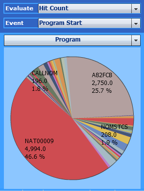
In the example above, the program NAT00009 started
4,994 times.
Use the following selections to find out:
| Evaluate: | Hit Count |
| Event: | Natural Statement |
| Criterion: | Program |
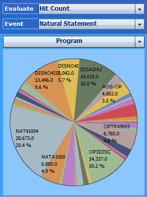
In the example above, the program NAT41004 executed
28,673 statement events.
Use the following selections to find out:
| Evaluate: | Hit Count |
| Event: | Program Load |
| Criteria: | Program, Target Program |
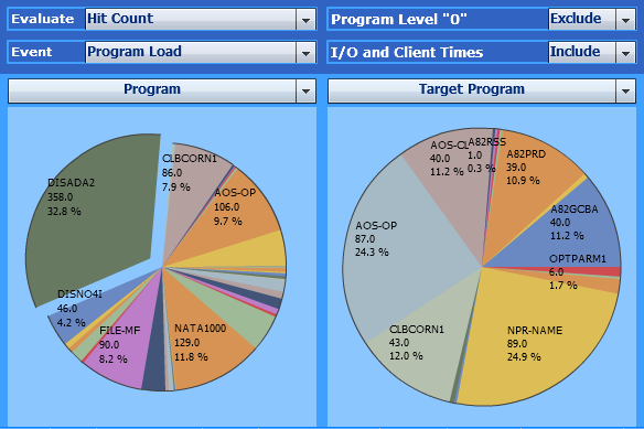
In the example above, the right pie chart shows the Natural objects
called by DISADA2. The Natural object NPR-NAME was
called 89 times.
Use the following selections to find out:
| Evaluate: | Hit Count |
| Event: | Program Load |
| Criteria: | Target Program, Program |
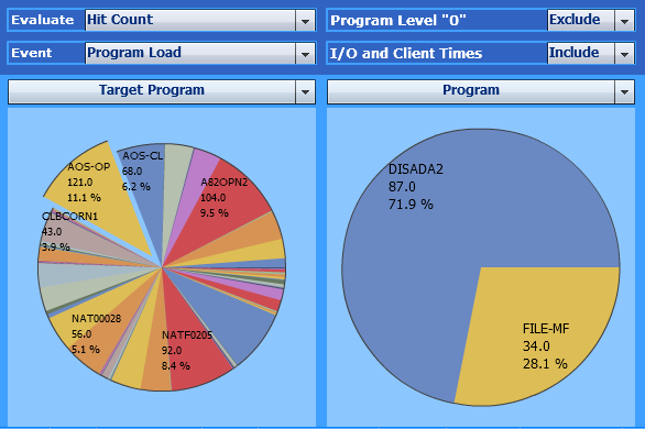
In the example above, the right pie chart shows the objects which
called the program AOS-OP. AOS-OP was called
87 times by the program DISADA2 and 34
times by the program FILE-MF.
Use the following selections to find out:
| Evaluate: | Hit Count |
| Event: | Runtime Error |
| Criteria: | Return Code, Library, Line, Statement |
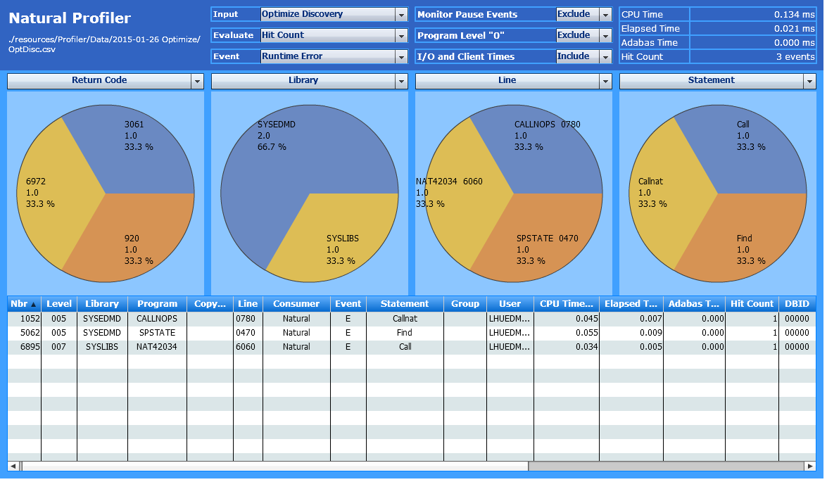
In the example above, the Hit Count in the page header indicates that three runtime errors occurred during application execution. The charts show which errors occurred, the library, program and line where they occurred, and the statements that caused the errors.