Add Key Performance Indicators (KPI)
Key performance indicators, or KPIs, are formats that can be conditionally applied to individual cells in a column or individual rows in the grid to indicate status or performance. You define the rules that determine whether formatting is applied and choose the formatting to apply if data meets the requirements of a given rule.
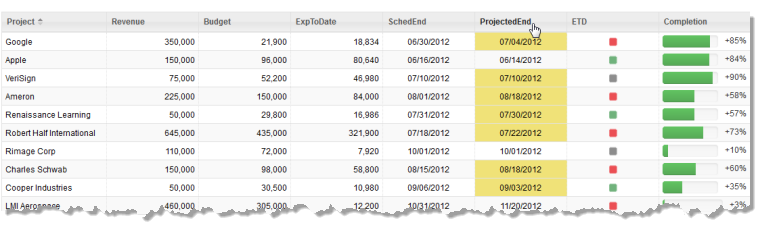
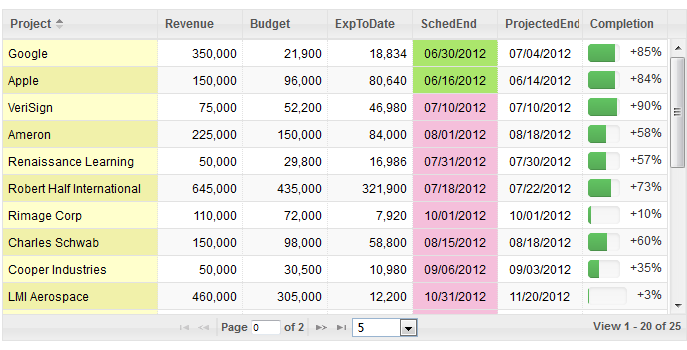
The previous example show two types of KPI formatting: icons in one column to indicate the expected delivery status for projects (on-time, late or early) and background colors in specific cells in another column indicating projects expected to finish in the current quarter.
To use KPI formatting for a grid
1. Select a column in the preview area or the Column list where you want to apply KPI formatting. For row formatting. select the column that should be used in rules to apply the KPI formatting.
2. Set the KPI option for the content.
3. Click Add KPI Rule in the bottom right corner of Data Configuration.
The View Maker wizard opens a KPI Rules area below the grid preview and Column Settings with a blank rule for this column.
4. Click Apply to save this rule and preview the effect.
See
Manage Rules and Conditions for other common KPI tasks.
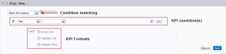
Define a KPI Condition
KPI conditions compare the values of one column to a single value or to the data in another column. You define the column to compare, the comparison to make and the value(s) to compare to in the:
 Left Field
 = the column with data to compare. Typically this is the column you have already selected in the preview area, but you can select another column if needed.
Middle Field = comparison to make.
is equal to,
is not equal to,
is less than,
is less than or equal to,
is greater than and
is greater than or equal to can be used for numeric or date data.
Note: | For correct numeric comparisons, both columns (left and right) in the condition must be numbers. In many cases, columns contain numbers but are considered Text. The easiest way to ensure this is to set Show As to Number. If both columns are not numeric, the comparison treats both as text which can cause errors. |
contains works for text fields and will match as long as the characters are found anywhere in column values. Comparison is
case sensitive.
Right Field = a single literal value or the name of another column with the values to compare to. Either:
Enter the single value to use in this field.
If this field has a list of columns, click

to return to edit mode where you can enter a value.
Click

to get different values from another column. Then select the column to use from the list of available columns.
Set Multiple KPI Conditions
Click
Add next to an existing condition to add another condition. Complete the fields (see
Define a KPI Condition for more information) for this new condition.
Change the condition matching rule to determine what is considered a match. Choose either Match All Conditions or Match Any Conditions.
Use KPI Icons
KPI Icons are useful to quickly define status or progress for a column based on conditions, such as the ETD column in this example:
The ETD column indicates whether the expected delivery date for a project is on-time

, early

or late

.
This example uses three rules, one for each icon:
You can have just the icons show or show both the data and the icons. You can also repeat icons to indicate rating or importance or use two or more different icons to indicate different conditions.
To use icons for KPI formatting
1. Set the Icon option.
2. Click Select Icon and either:
Select one of the built-in KPI icons and click
Close.
Or click the
Custom URL tab to use your own icon. Enter the URL to the icon image and click Close.
3. If you want to repeat this icon more than once, such as a rows of stars to indicate a rating, change the Repeat value.
4. Choose the icon placement and data visibility. Left or Right includes both the icon and the data. Centered shows just the icon.
5. To show other icons for this condition, click Add and repeat the steps to choose the icon, repetition and placement for another icon.
6. Click Apply.
Use KPI Cell Formatting
KPI cell formatting can change the background color, font color, font variation or font size for data in the selected column, such as this example:
This uses different background colors to indicate projects scheduled to be finished in the first two quarters versus projects scheduled for the last two quarters.
Note: | KPI cell formatting overrides both font formatting set in Column Settings and font formatting set in KPI rules with row formatting . |
To use KPI cell formatting
1. Set the Highlight Cell option.
2. Set any of the font options, as needed.
3. If needed, click Background and find the color you want to use as the background. Click Set this Color.
4. Click Apply.
Use KPI Row Formatting
KPI row formatting can change the background color, font color, font variation or font size for data in rows that match the condition(s) in the rule, such as this example which highlights project rows when the expected revenue is greater than $250,000:
Note: | KPI row formatting overrides font formatting set in Column Settings. It can be overridden, however by font formatting set in KPI rules with cell formatting . |
To use KPI cell formatting
1. Set the Highlight Row option.
2. Set any of the font options, as needed.
3. If needed, click Background and find the color you want to use as the background. Click Set this Color.
4. Click Apply.
Manage Rules and Conditions
You can also:
Open or collapse rules by clicking on the rule heading.
Remove a rule. Click the rule heading to open it, if needed, and click
Remove.
Remove a condition. Open the rule, if needed, and click
Remove next to the condition.
Note: | You cannot remove the very first condition. Instead, simply change the fields to match another rule and then delete the duplicate. |