Natural supports the processing of arrays. Arrays are multi-dimensional tables, that is, two or more logically related elements identified under a single name. Arrays can consist of single data elements of multiple dimensions or hierarchical data structures which contain repetitive structures or individual elements.
This document covers the following topics:
In Natural, an array can be one-, two- or three-dimensional. It can be an independent variable, part of a larger data structure or part of a database view.
Important:
Dynamic variables are not allowed in an array
definition.
![]() To define a one-dimensional array
To define a one-dimensional array
After the format and length, specify a slash followed by a so-called "index notation", that is, the number of occurrences of the array.
For example, the following one-dimensional array has three occurrences, each occurrence being of format/length A10:
DEFINE DATA LOCAL
1 #ARRAY (A10/1:3)
END-DEFINE
...
![]() To define a two-dimensional array
To define a two-dimensional array
Specify an index notation for both dimensions:
DEFINE DATA LOCAL
1 #ARRAY (A10/1:3,1:4)
END-DEFINE
...
A two-dimensional array can be visualized as a table. The array defined in the example above would be a table that consists of 3 "rows" and 4 "columns":
To assign initial values to one or more occurrences of an array, you use
an INIT specification, similar to that for
"ordinary" variables,
as shown in the following examples.
The following examples illustrate how initial values are assigned to a one-dimensional array.
To assign an initial value to one occurrence, you specify:
1 #ARRAY (A1/1:3) INIT (2) <'A'>
A is assigned to the second occurrence.
To assign the same initial value to all occurrences, you specify:
1 #ARRAY (A1/1:3) INIT ALL <'A'>
A is assigned to every occurrence. Alternatively, you
could specify:
1 #ARRAY (A1/1:3) INIT (*) <'A'>
To assign the same initial value to a range of several occurrences, you specify:
1 #ARRAY (A1/1:3) INIT (2:3) <'A'>
A is assigned to the second to third occurrence.
To assign a different initial value to every occurrence, you specify:
1 #ARRAY (A1/1:3) INIT <'A','B','C'>
A is assigned to the first occurrence, B to
the second, and C to the third.
To assign different initial values to some (but not all) occurrences, you specify:
1 #ARRAY (A1/1:3) INIT (1) <'A'> (3) <'C'>
A is assigned to the first occurrence, and C
to the third; no value is assigned to the second occurrence.
Alternatively, you could specify:
1 #ARRAY (A1/1:3) INIT <'A',,'C'>
If fewer initial values are specified than there are occurrences, the last occurrences remain empty:
1 #ARRAY (A1/1:3) INIT <'A','B'>
A is assigned to the first occurrence, and B
to the second; no value is assigned to the third occurrence.
This section illustrates how initial values are assigned to a two-dimensional array. The following topics are covered:
For the examples shown in this section, let us assume a two-dimensional array with three occurrences in the first dimension ("rows") and four occurrences in the second dimension ("columns"):
1 #ARRAY (A1/1:3,1:4)
| (1,1) | (1,2) | (1,3) | (1,4) |
| (2,1) | (2,2) | (2,3) | (2,4) |
| (3,1) | (3,2) | (3,3) | (3,4) |
The first set of examples illustrates how the same initial value is assigned to occurrences of a two-dimensional array; the second set of examples illustrates how different initial values are assigned.
In the examples, please note in particular the usage of the notations
* and V. Both notations refer to all
occurrences of the dimension concerned: * indicates that all
occurrences in that dimension are initialized with the same value,
while V indicates that all occurrences in that dimension are
initialized with different values.
To assign an initial value to one occurrence, you specify:
1 #ARRAY (A1/1:3,1:4) INIT (2,3) <'A'>
| A | |||
To assign the same initial value to one occurrence in the second dimension - in all occurrences of the first dimension - you specify:
1 #ARRAY (A1/1:3,1:4) INIT (*,3) <'A'>
| A | |||
| A | |||
| A |
To assign the same initial value to a range of occurrences in the first dimension - in all occurrences of the second dimension - you specify:
1 #ARRAY (A1/1:3,1:4) INIT (2:3,*) <'A'>
| A | A | A | A |
| A | A | A | A |
To assign the same initial value to a range of occurrences in each dimension, you specify:
1 #ARRAY (A1/1:3,1:4) INIT (2:3,1:2) <'A'>
| A | A | ||
| A | A |
To assign the same initial value to all occurrences (in both dimensions), you specify:
1 #ARRAY (A1/1:3,1:4) INIT ALL <'A'>
| A | A | A | A |
| A | A | A | A |
| A | A | A | A |
Alternatively, you could specify:
1 #ARRAY (A1/1:3,1:4) INIT (*,*) <'A'>
1 #ARRAY (A1/1:3,1:4) INIT (V,2) <'A','B','C'>
| A | |||
| B | |||
| C |
1 #ARRAY (A1/1:3,1:4) INIT (V,2:3) <'A','B','C'>
| A | A | ||
| B | B | ||
| C | C |
1 #ARRAY (A1/1:3,1:4) INIT (V,*) <'A','B','C'>
| A | A | A | A |
| B | B | B | B |
| C | C | C | C |
1 #ARRAY (A1/1:3,1:4) INIT (V,*) <'A',,'C'>
| A | A | A | A |
| C | C | C | C |
1 #ARRAY (A1/1:3,1:4) INIT (V,*) <'A','B'>
| A | A | A | A |
| B | B | B | B |
1 #ARRAY (A1/1:3,1:4) INIT (V,1) <'A','B','C'> (V,3) <'D','E','F'>
| A | D | ||
| B | E | ||
| C | F |
1 #ARRAY (A1/1:3,1:4) INIT (3,V) <'A','B','C','D'>
| A | B | C | D |
1 #ARRAY (A1/1:3,1:4) INIT (*,V) <'A','B','C','D'>
| A | B | C | D |
| A | B | C | D |
| A | B | C | D |
1 #ARRAY (A1/1:3,1:4) INIT (2,1) <'A'> (*,2) <'B'> (3,3) <'C'> (3,4) <'D'>
| B | |||
| A | B | ||
| B | C | D |
1 #ARRAY (A1/1:3,1:4) INIT (2,1) <'A'> (V,2) <'B','C','D'> (3,3) <'E'> (3,4) <'F'>
| B | |||
| A | C | ||
| D | E | F |
A three-dimensional array could be visualized as follows:
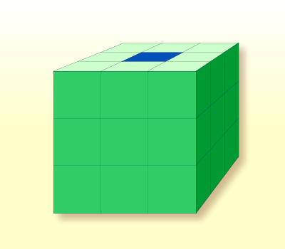
The array illustrated here would be defined as follows (at the same time assigning an initial value to the highlighted field in Row 1, Column 2, Plane 2):
DEFINE DATA LOCAL
1 #ARRAY2
  2 #ROW (1:4)
    3 #COLUMN (1:3)
      4 #PLANE (1:3)
        5 #FIELD2 (P3) INIT (1,2,2) <100>
END-DEFINE
...
If defined as a local data area in the data area editor, the same array would look as follows:
I T L Name                             F Leng Index/Init/EM/Name/Comment
- - - -------------------------------- - ---- ---------------------------------
    1 #ARRAY2
    2 #ROW                                    (1:4)
    3 #COLUMN                                 (1:3)
    4 #PLANE                                  (1:3)
I   5 #FIELD2                          P    3
The multiple dimensions of an array make it possible to define data structures analogous to COBOL or PL1 structures.
DEFINE DATA LOCAL
1 #AREA
  2 #FIELD1 (A10)
  2 #GROUP1 (1:10)
    3 #FIELD2 (P2)
    3 #FIELD3 (N1/1:4)
END-DEFINE
...
In this example, the data area #AREA has a total size
of:
10 + (10 * (2 + (1 * 4))) bytes = 70 bytes
#FIELD1 is alphanumeric and 10 bytes long.
#GROUP1 is the name of a sub-area within #AREA, which
consists of 2 fields and has 10 occurrences. #FIELD2 is packed
numeric, length 2. #FIELD3 is the second field of
#GROUP1 with four occurrences, and is numeric, length 1.
To reference a particular occurrence of #FIELD3, two
indices are required: first, the occurrence of #GROUP1 must be
specified, and second, the particular occurrence of #FIELD3 must
also be specified. For example, in an ADD statement later in the
same program, #FIELD3 would be referenced as follows:
ADD 2 TO #FIELD3 (3,2)
Adabas supports array structures within the database in the form of multiple-value fields and periodic groups. These are described under Database Arrays.
The following example shows a DEFINE DATA view containing a
multiple-value field:
DEFINE DATA LOCAL
1 EMPLOYEES-VIEW VIEW OF EMPLOYEES
  2 NAME
  2 ADDRESS-LINE (1:10) /* <--- MULTIPLE-VALUE FIELD
END-DEFINE
...
The same view in a local data area would look as follows:
I T L Name                             F Leng Index/Init/EM/Name/Comment
- - - -------------------------------- - ---- ---------------------------------
  V 1 EMPLOYEES-VIEW                          EMPLOYEES
    2 NAME                             A   20
  M 2 ADDRESS-LINE                     A   20 (1:10) /* MU-FIELD
A simple arithmetic expression may also be used to express a range of occurrences in an array.
Examples:
MA (I:I+5)
|
Values of the field MA are referenced, beginning
with value I and ending with value I+5.
|
MA (I+2:J-3) |
Values of the field MA are referenced, beginning
with value I+2 and ending with value J-3.
|
Only the arithmetic operators plus (+) and minus (-) may be used in index expressions.
Arithmetic support for arrays include operations at array level, at row/column level, and at individual element level.
Only simple arithmetic expressions are permitted with array variables, with only one or two operands and an optional third variable as the receiving field.
Only the arithmetic operators plus (+) and minus (-) are allowed for expressions defining index ranges.
The following examples assume the following field definitions:
DEFINE DATA LOCAL
01 #A (N5/1:10,1:10)
01 #B (N5/1:10,1:10)
01 #C (N5)
END-DEFINE
...
ADD #A(*,*) TO #B(*,*)
The result operand, array #B, contains the addition,
element by element, of the array #A and the original value of
array #B.
ADD 4 TO #A(*,2)
The second column of the array #A is replaced by its
original value plus 4.
ADD 2 TO #A(2,*)
The second row of the array #A is replaced by its
original value plus 2.
ADD #A(2,*) TO #B(4,*)
The value of the second row of array #A is added to the
fourth row of array #B.
ADD #A(2,*) TO #B(*,2)
This is an illegal operation and will result in a syntax error. Rows may only be added to rows and columns to columns.
ADD #A(2,*) TO #C
All values in the second row of the array #A are added
to the scalar value #C.
ADD #A(2,5:7) TO #C
The fifth, sixth, and seventh column values of the second row of
array #A are added to the scalar value #C.