A continuous-time value type, especially of the float (that is, numeric) type, is typically used to represent the measurement of some continuous physical quantity or property by a sensor. For example, a value may represent one of the following:

These are all continuous measurable properties which are analog in nature. There will be some degree of precision as to how accurately they can be measured in both time and value (and within physical limits). By time accuracy, we mean how frequently a measurement can be made and how precisely the time of the measurement is recorded. There may also be latency - a delay between a change in the actual property and when that can be measured. By value accuracy, we mean with what level of precision the value can be measured - typically at least 2 significant figures, and rarely more than 4 or 5 significant figures of precision can be distinguished. By continuous, we mean that it is valid to measure the property at any point in time.

Taking discrete measurements at different times rather than continuously may be referred to as sampling (see also https://en.wikipedia.org/wiki/Sampling_(signal_processing)), and limits as to the value precision may be referred to as quantization error (see also https://en.wikipedia.org/wiki/Quantization_(signal_processing)). When measuring a continuous value, the rate at which measurements are obtained should not make significant differences to the output of a block or a model. More measurements may give a more accurate output, but should not make a gross change to calculations.

For example, a sensor measuring the rotational speed of an axle may be able to provide a new measurement every one tenth (0.1) of a second, and only measure in the range 0 to 10000 rpm to the nearest 50 rpm. A change of 10 or 20 rpm may not result in any change of measured value, as the change is less than the level of precision. Applying brakes to a rotating axle to stop it may not be detected immediately, but result in one reading of 1000 rpm, followed by a reading 0.1 seconds later at 0 rpm after the axle has stopped (while the axle would take a few tens of milliseconds to stop, slowing down over that time period).

A sensor may be connected in such a way that it provides a new measurement at a regular frequency (for example, audio sampling at 8,000 Hz or a camera taking video at 50 frames a second). This is a regular sampling input.

A simple and common optimization is that a sensor or device may generate a new measurement value only if the value is different to the previous value. For many sensors, it would be normal to measure something that often maintains a steady or constant value (at least to within the quantization limit), and there is little value in repeatedly sending the same value. This is an on-change input. There will still be an underlying sampling frequency, but new values are only transmitted from the sensor if they are different.

It is also possible to combine the regular sampling and on-change forms together: a sensor that generates a new input if the measurement is different, or periodically. This is a hybrid input. For example, the rotational sensor described above may only send a value if the rotation speed changes, or every 10 seconds regardless.

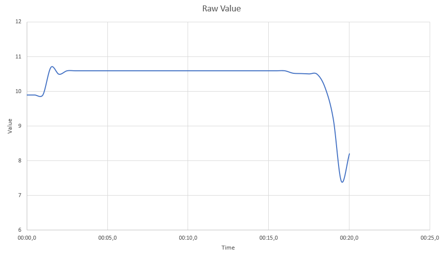
As an example, consider a raw value that changes over time as so:

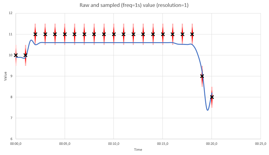
But suppose the sensor can only measure to the nearest whole number, and only once a second. The value thus has some error, shown by the red error bars:

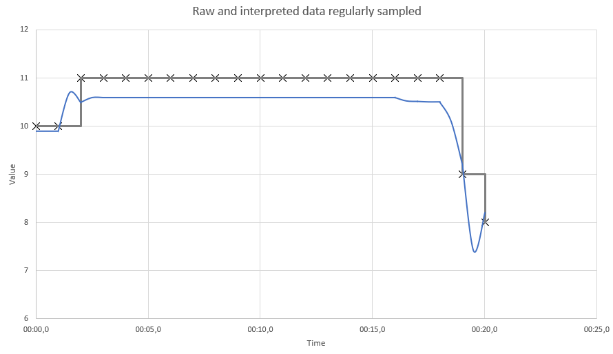
A regular sampling sensor would generate uniform inputs:

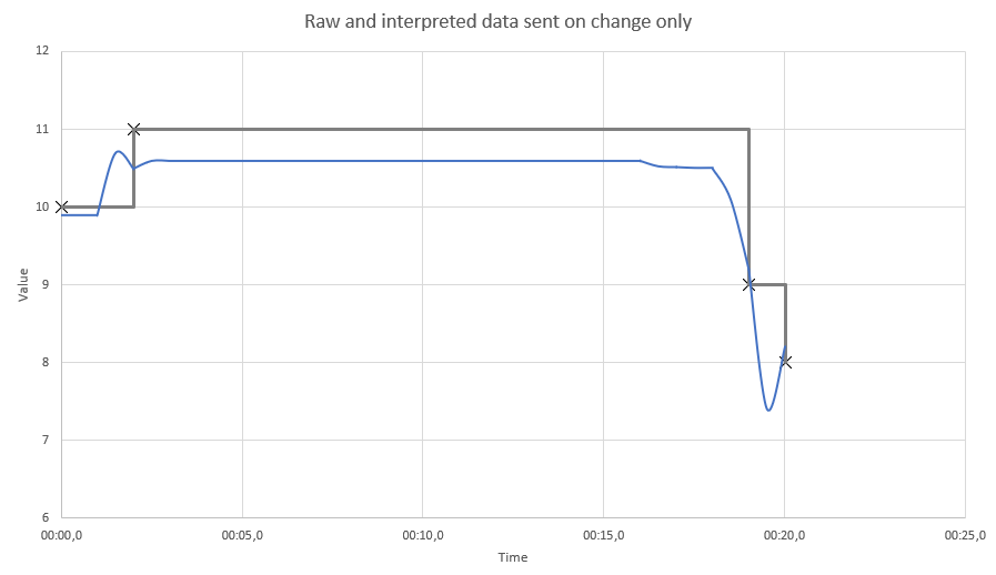
While an on-change sensor would generate inputs only when a value changes:

The grey line shows how a real-time processing system such as Apama interprets such values. A value is assumed to maintain the latest value until it is replaced by a newer value. It is also common to draw lines between measurements. So there is a straight line decreasing from value 11 at 00:01 to value 9 at 00:19. However, a real-time system cannot do this. It does not know what the next value is, whereby viewing historic data can interpolate between values. At time 00:19.5, the only information it has is that the value was 11 and then 9. It does not yet know that the value will be 8 at time 00:20. Note that there is no difference between the interpreted grey line in the regularly sampled and on-change-only case. Note that in the middle of the graph, there is a significant quantization error (the true value of 10.6 is read as 11), and the sampling frequency of only once a second means that the minimum point of 7.4 at 00:19.5 seconds is lost.